When we think about the classic model for dynamic programming, typically we think about first enumerating the state, and then enumerating the transitions from that state. But sometimes that perspective doesn’t yield itself to a sufficiently fast solution. Let’s look at some examples.

Bellman-Ford

Let’s begin with a classic example, the Bellman-Ford algorithm. The code for that typically looks something like this:

1
2
3
for (int iter = 0; iter < n - 1; iter++)
    for (auto [u, v, w] : edges)
        dist[v] = min(dist[v], dist[u] + w);

One perspective of this algorithm is that it is dynamic programming. Suppose there are no negative cycles, so the shortest distance from the source node $s$ to every other vertex in the same component is well-defined. Then each shortest path is always simple (no repeated vertices).

A simple path can contain at most $n$ vertices and therefore at most $n - 1$ edges. Initially, the only distance correctly computed is $dist[s] = 0$. In each iteration, we iterate over our edge list and perform what is known as a “relaxation”, where we update $dist[v]$ based on the shortest path to $u$, plus the edge from $u$ to $v$. The important thing is that after the first iteration, all shortest paths with one edge will be correctly computed. In general, after the $k$th iteration, all shortest paths with $k$ edges will be correctly computed, because prior to that iteration all shortest paths with $k-1$ edges were correctly computed, and every shortest path with $k$ edges consists of a $k-1$ length path plus an extra edge covered in the $k$th iteration. So after $n - 1$ iterations, all shortest paths with at most $n-1$ edges (all of them) will be correctly computed, so the algorithm is correct.

If we look at this through the lens of the classic dynamic programming model, what’s really happening here is there is an implicit second dimension. The actual state is $dp[k][v]$ denoting the shortest distance from $s$ to $v$ with at most $k$ edges. And the transition would be

The first part of that transition happens implicitly by reusing the same table for each iteration, and the second part of that transition is covered by the relaxation in each iteration. Bellman-Ford is essentially a memory efficient implementation of this recurrence.

If we code the DP explicitly with a 2D table, we get $\mathcal O(n(n + m))$. Compared to $\mathcal O(nm)$ Bellman-Ford, this way is worse when $m \ll n$.

DP to Maintain Convex Polygon

This is actually the problem that kickstarted this blog post. Problem K from the first stage of the 2022-23 Universal Cup gives us a simple polygon with $n \leq 200$ vertices and asks us to count the number of subsets of vertices (of size at least 2) such that for every pair of vertices in the subset, the line segment between them lies inside (or on the boundary of) the polygon.

We can start by precomputing for every pair of vertices whether or not the line segment between them lie inside the polygon in $\mathcal O(n^3)$. This subproblem itself is actually an ICPC World Finals problem, namely problem A from the 2017-18 WF, so you can refer to the solution to that for more details.

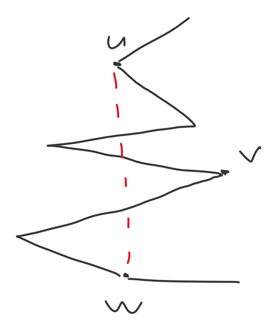
We can also observe that the subset of vertices we choose should form a convex polygon. If there are three adjacent vertices $u, v, w$ that form a concave section of the subset polygon, then some part of the line segment from $u$ to $w$ would lie outside the original polygon.

On the other hand, if the subset polygon is convex, then it suffices to check that the edges of that polygon lie within the original polygon, and we don’t have to check all pairs of vertices.

These observations alone bring us to an $\mathcal O(n^4)$ DP: $dp[s][u][v]$ denotes the number of subsets where the first vertex was $s$, the last 2 vertices taken were $u$ and $v$, and we have an $\mathcal O(n)$ transition for enumerating the next vertex to take. A transition to vertex $w$ is valid if $u \to v \to w$ is a counterclockwise turn. That’s not fast enough. But let’s consider what makes this DP redundant: storing both of the last 2 vertices in order to track whether or not the next turn is counterclockwise.

Instead, let’s redefine our DP: let $dp[s][v]$ denote the number of subsets where the first vertex was $s$ and the last vertex was $v$. And instead of iterating first state, then transition, let’s enumerate the transitions as the outer loop. Collect all vectors between all pairs of vertices (so an edge $uv$ is included twice, once as $u \to v$ and once as $v \to u$) and sort them based on polar angle. Now iterate over the vectors in that order, and when we encounter vector $u \to v$, iterate over all $s$ and perform a relaxation $dp[s][v] \mathrel{+}= dp[s][u]$. So the code would look something like this:

1
2
3
4
5
// vecs contains all vectors u -> v that lie within the original polygon
sort(vecs.begin(), vecs.end(), cmp);
for (auto [u, v] : vecs)
    for (int s = 0; s < n; s++)
        dp[s][v] += dp[s][u];

This is very clearly $\mathcal O(n^3)$. As for correctness, after processing the $i$th vector, all DP states will represent having built part of a polygon with the last edge at an angle no more than the angle of the $i$th vector. So the condition of enforcing counter-clockwise turns in our subset polygon is automatically satisfied by the order in which we process the vectors.

Now unfortunately, the code I wrote above wouldn’t actually get AC on the problem I linked, because the original problem allows collinear points, so you have to do some extra work to avoid reusing the same edge twice, once in each direction. But that’s an implementation detail and not the core idea behind the solution.

Again, if we were to look at this from the classic dynamic programming model perspective, there is an implicit extra dimension. Our actual state is $dp[i][s][v]$ denoting the number of subsets where we have processed up to the $i$th vector, the first vertex was $s$, and the last vertex was $v$. And simulating this DP directly would consume $\mathcal O(n^4)$ time. So by saving memory, we also saved complexity.

This particular DP for computing convex polygons has actually appeared in a number of other problems.

• Problem H: Satanic Panic from Codeforces (with explanation of the trick here)
• Problem F: Integer Convex Hull from AtCoder in $\mathcal O(n^3)$ instead of $\mathcal O(n^4)$
• Pegs from NENA 2013 in $\mathcal O(n^6)$ instead of $\mathcal O(n^8)$

Genius - A Codeforces Problem

Finally, this problem is probably the first time I truly saw this idea, and I remember reading the editorial at the time and thinking it looked very similar to Bellman-Ford.

IQ is always increasing, so one approach is $dp[i][j]$ denoting the maximum number of points if the last 2 problems you solved were $i$ and $j$. Your IQ would therefore be $|c_i - c_j|$. And you have $\mathcal O(n)$ transition by enumerating the next problem you solve with larger complexity gap and a different tag, giving an $\mathcal O(n^3)$ solution overall, which is too slow.

Similar to the geometry problem, we will change from storing the last 2 problems to just the last problem solved and instead enumerate the edges in a better order. Because $c_i = 2^i$, a gap $(i, j)$ is greater than gap $(k, l)$ for $i > j, k > l$ iff $i > k$ or $i = k, j > l$. So the correct order to enumerate these edges in to get increasing order gaps is increasing $i$ as the outer loop, then decreasing $j$ as the inner loop.

1
2
3
4
5
6
7
for (int i = 1; i < n; i++)
    for (int j = i - 1; j >= 0; j--)
        if (tag[i] != tag[j]) {
            long long di = dp[i], dj = dp[j];
            dp[i] = max(dp[i], dj + abs(s[i] - s[j]));
            dp[j] = max(dp[j], di + abs(s[i] - s[j]));
        }

The condition of enforcing increasing IQ is automatically taken care of by the order in which we enumerate these edges. Or alternatively, the dimension of current IQ has become an implicit dimension. So again, we cut memory to also cut complexity and get $\mathcal O(n^2)$.

More Problems

• Problem F: Brave CHAIN from AtCoder