A Shift in Perspective
I’ve seen numerous problems recently where the solution comes from a shift in perspective, and I’ve found them amusing enough to write a whole blog around this topic. I wouldn’t consider this a technique but rather just an explanation of visual intuition for problem solving.
Codeforces Round 767, Div 1 D2: Game on Sum (Hard Version)
Firstly, I will assume familiarity with the $\mathcal O(nm)$ DP solution that solves the Easy Version, which you can read about in the official editorial.
Let $dp[i][j]$ be the answer when there are $i$ turns left and Bob has to choose $j$ more add operations. The transitions are as follows:
\[\begin{align*} j = 0 &\implies dp[i][j] = 0 \\ j = i &\implies dp[i][j] = i \cdot k \\ 0 < j < i &\implies dp[i][j] = \frac{dp[i-1][j-1] + dp[i-1][j]}{2} \end{align*}\]Intuition for the DP
It would be ironic for a blog post about intuition to not explain the intuition for this recurrence. The editorial already covers the intuition pretty well, but I’ll include it here for sake of completeness.
Let’s knock out the straightforward cases first. If $j = 0$, the answer is $0$ because Bob can just subtract every time, so it would be suboptimal for Alice to pick any positive number. If $j = i$, the answer is $i \cdot k$ because Bob is forced to add for all of his remaining operations, so Alice can cash in a maximum of $+k$ on each operation.
Now let’s consider another small case like $i = 2, j = 1$. Say Alice picks $x$. If Bob subtracted $x$ now, he would have no subtract operations left and Alice would cash in $+k$ in the final operation, so the resulting score would be $k - x$. If Bob added $x$ now, he would be able to subtract on his final operation and Alice would optimally state $0$ as her final number, so the resulting score would be $x$. Since Bob wants to minimize the score, he would pick the choice resulting in $\min(x, k - x)$. Now Alice wants to pick the $x$ that maximizes this minimum. The function is maximized when $x = k - x$, or $x = \frac{k}{2}$, and the final score would be $\frac{k}{2}$.
There’s no reason we can’t extend this logic to the general case. Say we’re at any arbitrary state of the game $(i, j)$. If Alice selects $x$, Bob makes the choice that attains $\min(dp[i-1][j] - x, dp[i-1][j-1] + x)$1. For Alice to maximize this minimum, she selects the $x$ such that $dp[i-1][j] - x = dp[i-1][j-1] + x$, or $x = \frac{dp[i-1][j] - dp[i-1][j-1]}{2}$. The final score would be $\frac{dp[i-1][j-1] + dp[i-1][j]}{2}$. You can prove that this is always a valid move (i.e. $0 \leq \frac{dp[i-1][j] - dp[i-1][j-1]}{2} \leq k$) with some induction and algebra (written out in detail in this comment).
- I always find DP solutions for game theory problems humorous because it's funny to imagine Alice and Bob mentally computing DP tables in their head while playing a game with each other. ↩
Ok, now we must solve the hard version with constraints $m \leq n \leq 10^6$. To me, it isn’t immediately obvious how to optimize this DP to linear time just by staring at the formulas. So as the title suggests, it’s time for a shift in perspective!
Let’s draw out the DP table, because visualizing stuff is great.
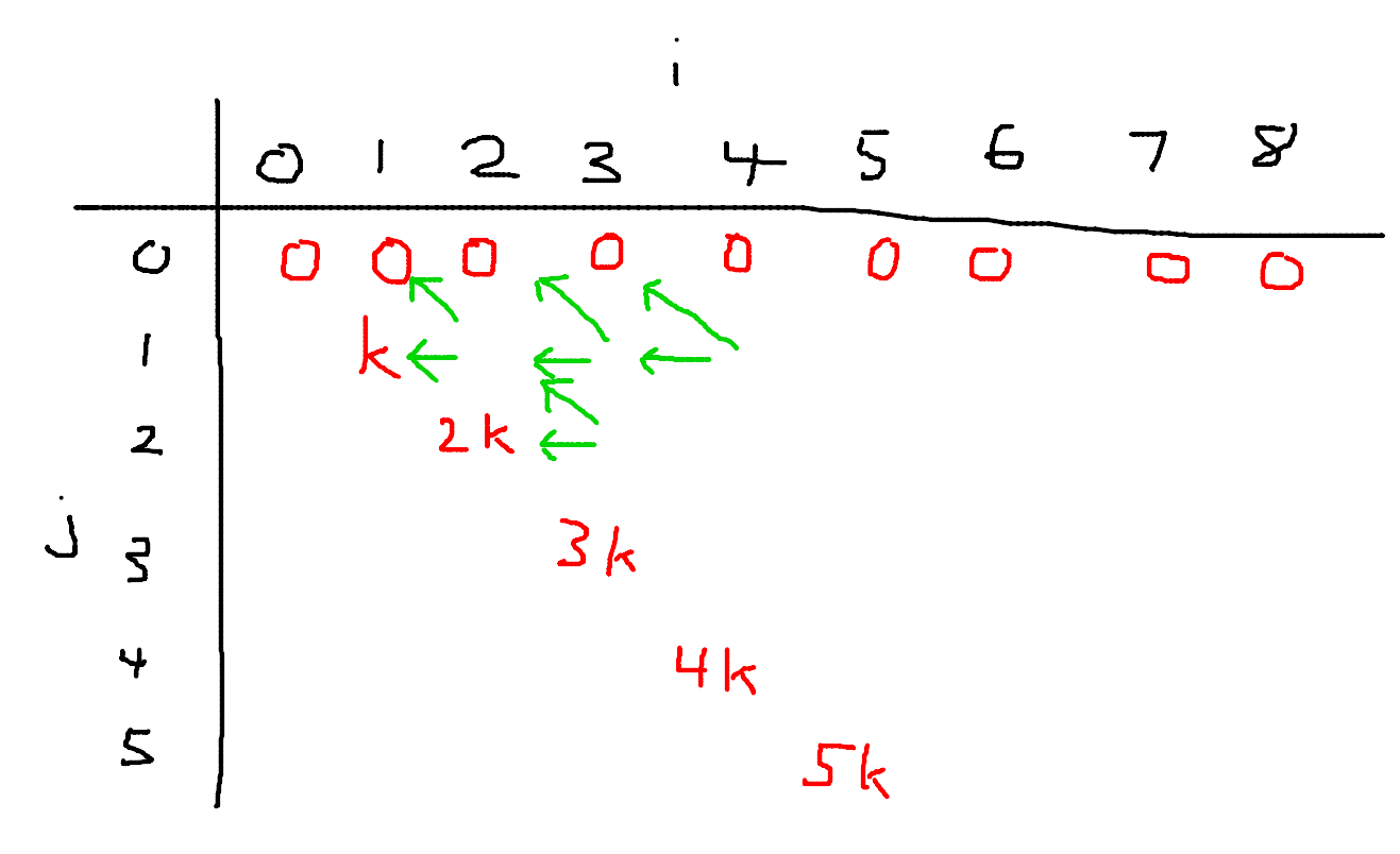
You know, I’m something of an artist myself.
Yes, I realize I have $i$ as the columns and $j$ as the rows in this diagram, but just roll with it. Each cell $(i, j)$ contains the value of $dp[i][j]$. So for cells of the form $(i, 0)$, their values are $0$. For cells of the form $(i, i)$, their values are $i \cdot k$. And for the remaining cells, I’ve drawn two green arrows representing the transitions from $(i, j)$ to $(i - 1, j)$ and $(i - 1, j - 1)$. Now here’s the cool part: since this looks like a grid, let’s think about grid paths. Say we initially start at cell $(n, m)$. We have a $\frac{1}{2}$ probability of moving to the cell on the left or diagonally up and left. If we ever reach a cell of the form $(i, i)$, we gain value $i \cdot k$ and stop moving. Now this problem becomes calculating the expected value of any path we take starting from $(n, m)$. Pretty neat!
This new interpretation is much easier to come up with an $\mathcal O(n)$ solution to. We precompute factorials and powers of $2$, and we iterate over each of the ending cells. If we end at $(i, i)$, we will take $n - i$ steps and move up exactly $m - i$ times. There are $\binom{n - i}{m - i}$ such paths, and we multiply by $\left(\frac{1}{2}\right)^{n - i}$ for the probability of making the right decision at each step. But this isn’t exactly correct, because we have to exclude the paths that go through cell $(i + 1, i + 1)$. So we subtract $\binom{n - i - 1}{m - i - 1}$ from our number of paths. The final answer is thus
\[\sum_{i=0}^m \left(\binom{n - i}{m - i} - \binom{n - i - 1}{m - i - 1}\right) \cdot \left(\frac{1}{2}\right)^{n - i} \cdot i \cdot k \\ = \sum_{i=0}^m \binom{n - i - 1}{m - i} \cdot \left(\frac{1}{2}\right)^{n - i} \cdot i \cdot k\]In summary, we’ve optimized a DP solution by looking at it under a combinatorics lens!
Kotlin Heroes Episode 8 G: A Battle Against a Dragon
I already wrote about this problem 4 months ago, but I’m mentioning it again as another example of a shift in perspective. The naive $\mathcal O(nm)$ DP approach is $dp[i][j] = \max(dp[i-1][j] + a[i][j], dp[i-1][j+1])$, where $dp[i][j]$ is the maximum damage done by the first $i$ warriors with $j$ barricades left and $a[i][j]$ is the amount of damage the $i$th warrior can do if there are exactly $j$ barricades. Again, optimizing this DP is best understood if you draw out the DP states on a grid, because then you’ll notice that the transitions can be expressed as 2D triangle queries and the problem becomes a data structures exercise. You can read more details in my older post about this problem.
Data Structures Note
I realized I never explained how to actually solve the “data structures exercise” at hand in my older post. So I’ll briefly explain it here. Treat the inputs as 2D points $(i, b_{ij})$ and sort them based on the diagonal $i + b_{ij}$ they lie on. Now perform a linesweep from smaller to larger diagonals and for each point, perform the following steps:
- Calculate its DP value by querying in a segment tree on the range $[b_{ij}, m]$.
- Insert the point into the segment tree at index $b_{ij}$.
By considering points in diagonal order, only points below the diagonal of the current point we’re considering will have already been inserted into the data structure, giving us the desired triangle query.
2019-2020 ICPC Southern and Volga Russian Regional Contest D: Conference Problem
Bounds are small which usually signify a DP solution is worth thinking about. However, the intervals are kind of annoying and don’t easily lend themselves to a recurrence in my opinion. We will eventually arrive at a recurrence that can be explained using the intervals, but here’s another way of arriving at it with a shift in perspective:
Let’s turn to the 2D plane (Noticing a theme here? I get all of my intuition from drawing stuff as geometric points or grids). Express an interval $[l, r]$ as a 2D point $(l, r)$. Another interval $[l’, r’]$ intersects $[l, r]$ if $l’ \leq r$ and $r’ \geq l$. In other words, the point $(l’, r’)$ lies to the upper left of the point $(r, l)$.
Now, let’s treat the countries as colors. So we can reformulate this problem as the following:
You are given $2n$ 2D points, some already colored. The points come in pairs of $(l, r)$ and $(r, l)$. We will refer to the $(l, r)$ points as “regular points” and $(r, l)$ points as “query points.” Points in the same pair must be the same color. Denote a query point as “bad” if it contains no different colored regular points to its upper left. Assign colors in the range $1 \dots 200$ to the uncolored points to maximize the number of bad points.
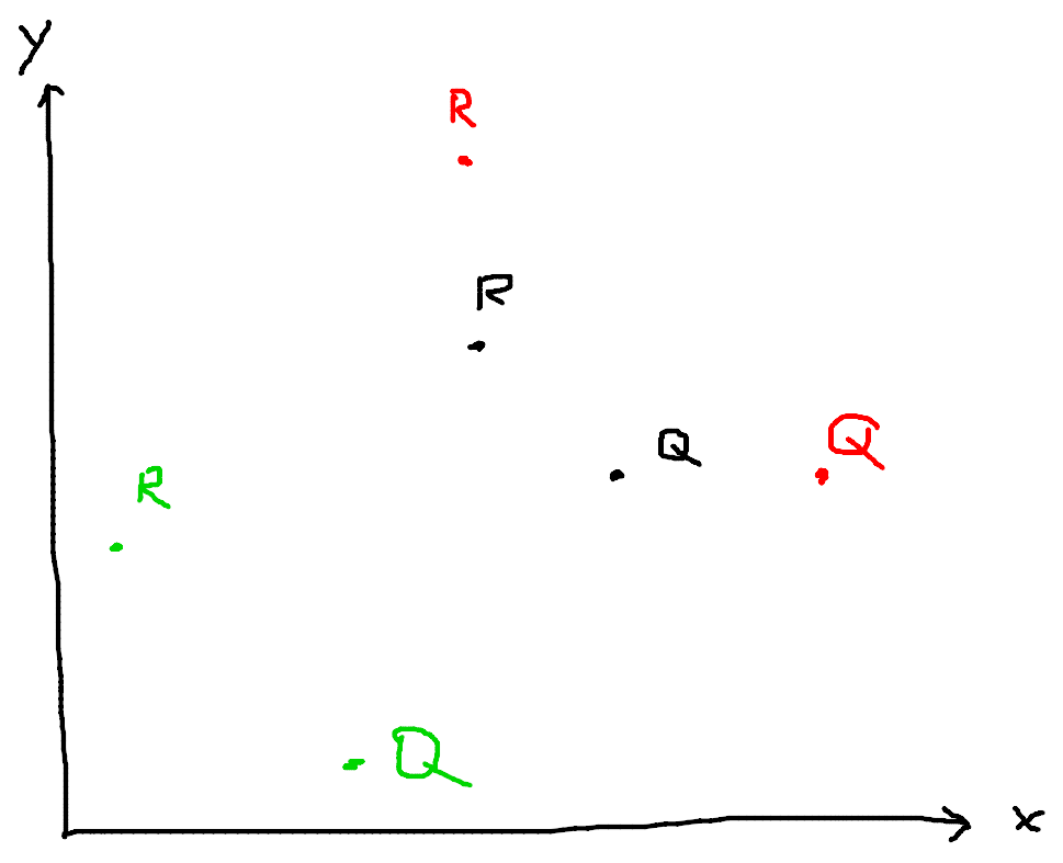
In this diagram, I’ve labeled the regular and query points with R and Q respectively. I used different colors to distinguish points with different c values. In this example, only the green point is bad, so our answer is 1.
Finally, here’s the observation that leads to our DP: Peform a linesweep to process the points from left to right. We only care about the y-coordinate of the highest two previously processed regular points of different colors. If we have a regular point with $c = 1$ at $y = 10$ and a regular point with $c = 2$ at $y = 9$, we couldn’t care less if there’s a regular point with $c = 3$ and $y = 7$, because any query point containing that third point in its upper left will also contain the first two points and thus already be guaranteed to have a point of different color in its upper left. Armed with that knowledge, we can formulate an $\mathcal O(n^3 C^2)$ solution: let $dp[i][j][k][l][m]$ be the maximum number of bad points if we’ve processed the first $i$ points, our highest regular point is at coordinate $j$ with color $k$, and our second highest regular point with a different color than the first is at coordinate $l$ with color $m$. Note that we’ve compressed our coordinates down to just $\mathcal O(n)$ distinct values instead of $10^6$.
We can do better. Storing the highest point is unnecessary, because we know that if our query point y-coordinate is below the y-coordinate of the second highest point of a different color, then we cover at least two distinct colors, and otherwise we only cover one color. So we can knock off two dimensions from our DP and get $\mathcal O(n^2 C)$ which fits under the constraints of this problem. One more note: we will instead store the lowest y-coordinate $j$ such that all regular points above $j$ are color $k$. In other words, we will store the lowest point of the highest color instead of the highest point of the second highest color. This is so we can determine if a query point is bad or not if its y-coordinate is greater than or equal to $j$.
To summarize, our $\mathcal O(n^2 C)$ DP is as follows: $dp[i][j][k]$ is the maximum number of bad points if we’ve processed the first $i$ points and all points with y-coordinate greater than or equal to $j$ are color $k$.
The transitions aren’t exactly straightforward, but they’re also not too hard and can be worked out with enough conviction and casework. I’ll leave the transitions as an exercise to the reader 🙂.
Boooo!
Ok fine. I really don’t feel like typing out the transitions because it’s just casework about if point $i$ is above or below $j$ and if it matches or doesn’t match color $k$. I’ll link a submission for reference and if you’re still confused you can leave a comment below. In my code I used a binary indexed tree for convenience, but it’s unnecessary because bounds are small enough that you can do everything with for loops.
Finale: Optimizing Bitmask DP with Graph Interpretation
I don’t have an official problem link for this problem, but it’s problem 6 on this blog. I usually don’t pay attention to blog posts about coding interview problems, but I read problem 6 and felt solving it for $n \leq 20$ was kind of non-trivial. Maybe I’m wrong and the solution is standard for others.
The problem is as follows:
You’re given two arrays $a$ and $b$, both of size $n$. In one operation, you can choose an integer $x$ and two indices $i$ and $j$, then add $x$ to $a_i$ and subtract $x$ from $a_j$. Find the minimum number of operations to transform array $a$ into $b$, or print $-1$ if it’s not possible.
Constraints: $n \leq 20, -10^9 \leq a_i, b_i \leq 10^9$
(The constraints on $a_i$ might be smaller, but I can’t read the image in the blog post very clearly and the complexity won’t depend on $a_i$ anyways.)
If the sum of $a_i$ and the sum of $b_i$ are not equal, then the answer is obviously $-1$ because the sum of $a_i$ remains constant after each operation. Otherwise, it’s always possible. Select some index $i$, add $b_i - a_i$ to $a_i$ and subtract $b_i - a_i$ from some other arbitrary $a_j$, then delete $a_i$ and $b_i$ from their respective arrays and solve the problem recursively. This procedure also provides an upper bound of $n - 1$ on the number of operations we perform.
To reduce the number of operations, we can partition the set of indices $U = \{1, 2, \dots, n\}$ into disjoint subsets, where for each subset $S$ is good. We define a subset $S$ to be good if $\sum_{i \in S} a_i = \sum_{i \in S} b_i$. Now we can fix the entire array just by performing our above procedure on each individual subset of indices. A subset $S$ can be fixed in $|S| - 1$ operations using the above procedure. So the answer is just $n - k$ where $k$ is the maximum number of disjoint subsets we can partition into.
This problem can be solved with a standard $\mathcal O(3^n)$ bitmask DP: let $dp[S]$ denote the maximum number of disjoint good subsets $S$ can be partitioned into. Iterate over all submasks and transition from that submask. Specifically:
\[dp[S] = \max_{S' \subset S, S' \text{ is good}} (dp[S \setminus S'] + 1)\]The answer is $n - dp[U]$. But $\mathcal O(3^n)$ is too slow for $n \leq 20$. Can we do better?
Here’s the key observation: if $S$ is good, and $S’ \subset S$ is good, then $S \setminus S’$ is also good. So instead of finding a partition of $U$ into disjoint subsets, let’s find a sequence of good subsets $S_1, S_2, \dots, S_k$ such that $S_1 \subset S_2 \subset \dots \subset S_k \subset U$. Now just take set differences between adjacent subsets in the sequence and we have our partition of disjoint good subsets!
It’s more clear how to optimize finding a maximum length sequence $S_1 \subset S_2 \subset \dots \subset S_k \subset U$. Let’s take a shift in perspective! Let’s treat all the good subsets as nodes in a graph, and draw an edge from $S$ to $T$ if $S \subset T$. We want to find a maximum length path from $\emptyset$ to $U$. However, this graph still could have up to $\mathcal O(3^n)$ edges. Instead, let’s also add in the non-good subsets as nodes so that now every subset of $U$ is a node and there are $2^n$ nodes. And instead of adding edges for all subset relations, just add an edge from a subset to every other subset with exactly one new bit turned on (i.e. we draw an edge from $S$ to $T$ if $S \subset T$ and $|T \setminus S| = 1$). This way, all subset relations are represented indirectly as nodes being reachable in this graph. Each node only has at most $n$ outgoing edges for each of its bits, so there are $\mathcal O(n \cdot 2^n)$ edges in this graph. And we can find the path with the maximum number of good nodes on it with DP, since it’s a directed acyclic graph. So we’ve successfully solved the problem in just $\mathcal O(n \cdot 2^n)$!
This blog post could go on forever because there are an infinite number of problems that benefit from shifting perspectives. In fact, sometimes problemsetters even start with a clear perspective, but then intentionally present you with a different perspective to hide the solution (e.g. the trick of this AtCoder problem is to flip A and B in the odd positions, which makes the operations much clearer). These perspective shifts aren’t meant to be black magic; I’m a huge proponent of visuals, and I typically find intuition just by drawing stuff. For example, if I’m doing a problem about arrays and intervals, you might see this on my paper:
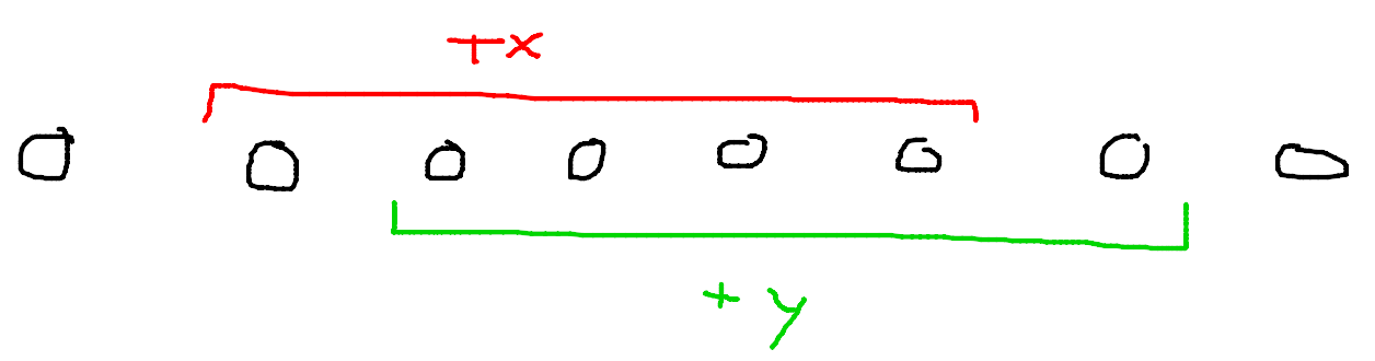
I can’t believe I’m providing such high quality diagrams for free 🙄
Thanks for reading. If you have any other cool problems, feel free to share!