Kruskal Reconstruction Tree
The Kruskal Reconstruction Tree (KRT) is something that is prevalent in folklore but scarcely documented, and most high rated users have probably either used this trick inadvertently or know of some other way of solving the problems that this DS solves. The most complete resource I know of is this CF blog, and this blog is basically me adding a few more uses of this DS that I’ve seen since the other blog was published. There’s also something similar called a line tree which seems to solve the same class of problems, but has a slightly different construction (an array instead of a tree). The name “Kruskal Reconstruction Tree” is one that I’ve heard others refer to it as, and is mentioned here.
The Concept
Let’s say we want to preprocess some tree in $\mathcal O(n \log n)$ and answer path max queries in $\mathcal O(1)$. Most people might answer queries in $\mathcal O(\log n)$ with binary lifting or even $\mathcal O(\log^2 n)$ with HLD. But how to do $\mathcal O(1)$? This blog contains a bunch of cool methods, one of which is the aforementioned line tree and one of which is KRT.
The KRT construction is as follows: start with a DSU containing $n$ isolated vertices and process the edges in increasing order of weight. When we insert a new edge $(u, v)$, we create a new vertex representing that edge and set it as the parent of $u$ and $v$’s components in the DSU. The initial sort of edges is $\mathcal O(n \log n)$ and we build the structure using a DSU with path compression (but not union by size/rank, as we care about parent-child relationships!), so the overall build time is $\mathcal O(n \log n)$. Our final KRT will have $2n - 1$ edges ($n$ vertices as leaves, and $n - 1$ vertices representing tree edges). Take a look at the diagrams below for a concrete example.
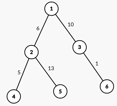
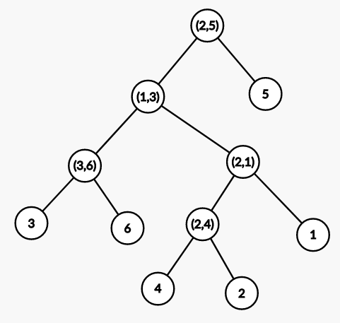
The original tree is on the left and its KRT is on the right. All newly created vertices representing edges are labelled with the pair of vertices they connect in the original tree.
From the diagram, we can discern a key property of the KRT: the maximum edge between $u$ and $v$ is their LCA in the KRT! It’s well-known how to compute LCA in $\mathcal O(1)$ using euler tour and RMQ, so we’ve successfully answered path max queries in $\mathcal O(1)$. The code is super simple:
Code
1
2
3
4
5
6
7
8
9
10
11
12
13
14
15
16
17
18
// id is the next unused id to assign to any new node created
// par is the standard definition of dsu parent
// adj will store the KRT
int id, par[2 * MAXN];
vector<int> adj[2 * MAXN];

int find(int u) {
    return par[u] == u ? u : par[u] = find(par[u]);
}

void unite(int u, int v) {
    u = find(u), v = find(v);
    if (u == v)
        return;
    par[u] = par[v] = par[id] = id;
    adj[id] = {u, v};
    id++;
}
Let’s now look at some real applications of this DS!
Codeforces Round 809, Div 2 E: Qpwoeirut and Vertices
Statement: Given an undirected graph, answer queries of the form $(l, r)$ where we find the smallest $k$ such that edges $1, \dots, k$ are sufficient for all vertices $l, \dots, r$ to be connected.
If we build the KRT, then the answer is simply the LCA of all vertices $l, \dots, r$. Of course, finding the LCA of a group of nodes by iterating over each of them is too slow. However, it suffices to find the nodes with the smallest and largest DFS times and take the LCA of those two nodes to get the LCA of the entire group. So the full solution is to build an RMQ on indices to query for the smallest and largest DFS times (in the KRT, not the original tree) within some range $[l, r]$, and then query the KRT to find the LCA edge, giving us an $\mathcal O((n + m) \log n + q)$ solution.
Codeforces Round 767, Div 1 E: Groceries in Meteor Town
Statement: Given a weighted tree with all nodes initially deactivated, answer queries of three types:
- Activate all nodes in some range $[l, r]$.
- Deactivate all nodes in some range $[l, r]$.
- For some node $x$, find the maximum weight edge from $x$ to any activated node.
Build the KRT again. That third query is simply asking for the LCA of all activated nodes and $x$. We can use the same trick as the previous problem. It suffices to find the activated node with the smallest and largest DFS times, and take the LCA of those nodes and $x$, to get the LCA of $x$ and all activated nodes. So we simply need a data structure that can range activate, range deactivate, and query for the minimum and maximum DFS times among all activated indices, which sounds like a job for a segment tree. Bam, Div 1E has never been so clean!
Codechef TULIPS: Tiptoe Through the Tulips
Statement: Given a weighted tree with all nodes initially containing a tulip, answer queries of the form $(d, u, k)$ where on day $d$, we perturb all nodes reachable from $u$ via edges with weight $\leq k$ and collect tulips from all nodes with tulips, and we want to know how many tulips we collect on that day. After a node is perturbed, it grows a tulip if it remains unperturbed in the next $X$ days.
Here we discover the true potential of KRT: we can turn component queries into subtree queries. Once the KRT is built, the set of nodes reachable from $u$ via edges with weight $\leq k$ correspond to a subtree in the KRT. To find the root of that subtree, we need to find the highest ancestor of $u$ with edge weight $\leq k$, which can be done using binary lifting as the edge weights increase monotonically going up the KRT. And if some DFS times are assigned, then subtree queries become range queries!
Now that we’re in the realm of range queries, we can explore our vast toolbox of range query structures. We need some data structure that can count indices in a range with time $\leq d - X$ and range set times to $d$. That’s an annoying formulation, so let’s consider a simpler one: count zeros in a range and range add. Whenever we process a query, we count zeros in that range, and then we add $1$ to that range and mark a future event to be processed at time $d + X$ to add $-1$ from that same range. This is much more tractable, as values are always non-negative so counting zeros is equivalent to counting minimums, so all necessary operations can be handled by segment tree.
IOI 2018: Werewolf
Statement: Given an undirected graph, process queries of the form $(S, E, L, R)$ where we want to know if it’s possible to reach $E$ from $S$ by first going through vertices with indices $\geq L$, reaching some vertex with index in between $[L, R]$, and going through vertices with indices $\leq R$.
It would be sacrilegious to talk about KRT and not mention the problem that spurred the trick, IOI Werewolf. So let’s look at this problem now. This time, our KRT is going to look a little different, since our edges are unweighted. For processing $\geq L$ ($\leq R$ is analogous), start with an empty DSU and process the vertices in decreasing order of index. When we process a vertex, find the components of all previously processed vertices and create a new vertex as the DSU parent of all of those components. Now for a query $S$, the set of vertices it can reach that are $\geq L$ correspond to some subtree in the KRT.
If we build two KRTs, one for $\geq L$ and the other for $\leq R$, then we can find the sets of vertices reachable from $S$ and $E$ that are $\geq L$ or $\leq R$ respectively, and then check if those sets intersect. Since these are subtree queries, we can again turn them into range queries with DFS times, and the problem reduces to the following: given two permutations $A$ and $B$, answer queries of checking if there exists a common element between $A[l_1, r_1]$ and $B[l_2, r_2]$.
This can be formulated as a sweepline problem. We can find something stronger, the count of common elements between $A[l_1, r_1]$ and $B[l_2, r_2]$. This equals the count of common elements between $A[l_1, r_1]$ and $B[1, r_2]$ minus the count of common elements between $A[l_1, r_1]$ and $B[1, l_2 - 1]$. So we sweep on $B$, and when we process an element, add $1$ to its corresponding position in $A$ in a binary indexed tree. Then, when we reach the right endpoint of a query in $B$, answer it by querying for the sum between $[l_1, r_1]$ in $A$ with the binary indexed tree. Voilà!
Closing
The power of KRT is giving us a way to handle queries based on partitioning components by edge weights into tree queries, something we are more familiar with and have more tools for. Of course, often times these queries can also be processed offline and answered while merging in DSUs, but that method isn’t always nice, and the KRT gives us a clean online method of answering them.