The trick for any segment tree problem is the following:

1. Figure out what information we need to store in the nodes.
2. Figure out how to combine two nodes.

In this case, it might help to start with thinking about how combining two nodes works, as that will guide us to know what info we need to maintain. Let’s say we’re considering the node representing range $[l, r]$ which is merged from two child nodes $[l, m]$ and $[m + 1, r]$, where $m = \lfloor \frac{l + r}{2} \rfloor$. The maximum subarray sum in $a[l, r]$ could fall into one of three cases:

1. It lies solely in the range $[l, m]$.
2. It lies solely in the range $[m + 1, r]$
3. It exists in both halves.

In the first and second case, we just take the maximum subarray sum computed in the child nodes. In the third case, the optimal subarray would consist of some suffix of the range $[l, m]$ and some prefix of the range $[m + 1, r]$. We can also compute the maximum prefix and suffix sum for each node, so that case 3 is simply reduced to the maximum suffix in the left child plus the maximum prefix in the right child. So this tells us what info we need to store in each node: the maximum subarray sum, the maximum prefix sum, the maximum suffix sum, and the total sum. We get the following method for updating:

1
2
3
4
5
6
7
// in my template the function signature is pull(a, b), but I'm using merge(left, right) here instead for clarity
void merge(Node left, Node right) {
    maxSum = max({left.maxSum, right.maxSum, left.maxSuffix + right.maxPrefix});
    maxPrefix = max(left.maxPrefix, left.sum + right.maxPrefix);
    maxSuffix = max(right.maxSuffix, right.sum + left.maxSuffix);
    sum = left.sum + right.sum;
}

Be careful that you handle ranges of all negative numbers correctly, because the problem does not allow for non-empty subarrays.

The extra condition of ignoring duplicates makes a direct online approach with segment tree difficult, because we don’t have a concise way of maintaining the set of all elements that have at least one occurrence in each node. So let’s consider an offline approach.

There’s a general sweepline approach for solving range query problems offline: sweep from left to right while updating some sort of data structure. When you encounter the right endpoint of some query, use the data structure to find the answer for that query.

In this case, our data structure will be an array $p$, where $p_i$ represents the maximum subarray sum excluding duplicates with left endpoint beginning at index $i$. We will also maintain an array $last_x$ storing the rightmost index with value $x$ in the array that we’ve encountered in our sweepline so far.

Let’s see what happens when we encounter $a_i$ in our sweepline. $a_i$ could contribute to every subarray beginning at $last_{a_i} + 1, last_{a_i} + 2, \dots, i$. It cannot contribute to a subarray beginning at $last_{a_i}$ or earlier, since such a subarray would already contain a copy of $a_i$ at index $last_{a_i}$ if it were to also include $a_i$, and duplicate elements only get added once. So we perform the following update:

1
2
3
4
for (int index=last[a[i]]+1; index<=i; index++) {
    sum[index] += a[i];
    p[index] = max(p[index], sum[index]);
}

Then, when we encounter some query $(l, r)$, its answer is simply

This offline algorithm runs in $\mathcal O(n(n + q))$, so let’s now boost the efficiency to $\mathcal O((n + q) \log n)$ by upgrading $p$ to a segment tree. We need a segment tree that can handle the following operations:

1. Add $x$ to all $a_i$ in some range.
2. Query for the maximum $p_i$ in some range.

After every operation, $p_i := \max(p_i, a_i)$, so $p_i$ is the maximum of all values $a_i$ ever changed into.

Believe it or not, this is possible with a segment tree, and is described in the “Historic Information” section of this segment tree beats tutorial.

That’s it! We’ve successfully solved this problem in $\mathcal O((n + q) \log n)$. Personally, I think this is the hardest GSS problem out of the entire series.

This is just GSS1 with updates. The update method doesn’t change any of the above logic.

The first operation is difficult to handle with traditional lazy propagation, because it’s not clear how applying the square root operation to a subarray affects the sum of that subarray. Let’s consider the naive way of updating the segment tree: we traverse all the way down to each leaf node in the range and update them directly, giving us $\mathcal O(n)$ per query. While that’s obviously too slow, it’s actually not far off from the right idea.

We will use the same idea as segment tree beats (don’t worry, this is easier than the proof for segment tree beats). Observe that for $a_i \leq 10^{18}$, we can only apply $a_i := \lfloor \sqrt a_i \rfloor$ 6 times before $a_i$ converges to 1. So let’s say you’re currently at some node, and you want to apply the square root operation to all elements in the range covered by that node. If all the elements are 1, applying the square root operation on them again is useless, so we can just stop traversing further.

Let’s prove a bound of $\mathcal O((n + m) \log n)$ from that optimization. Consider the following diagram:

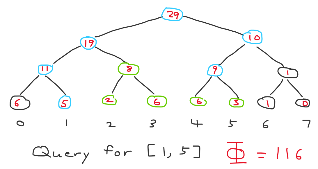
We will refer to the blue nodes as ordinary nodes and the green nodes as extra nodes (the same terminology used in the segment tree beats blog). Ordinary nodes are nodes we would visit in standard segment tree anyways. In the naive algorithm, we would also visit all the extra nodes, which could be $\mathcal O(n)$ per query. We will keep some counter on each leaf node representing how many more times we can apply the square root operation to that element before it reduces to 1 (the red numbers in the diagram). The counter can be at most 6 for each leaf node. Finally, we keep some counter on each non-leaf node that equals the sum of the counters of its children. Let $\Phi$ equal the sum of all counters written on all nodes in the tree. What is the initial value of $\Phi$? It is $\mathcal O(n \log n)$.

The number of ordinary nodes we visit is $\mathcal O(m \log n)$, since that’s just standard segment tree. Under what cases will we visit an extra node? We visit an extra node whenever there exists a non-one element in that subtree, aka if the counter on the extra node is positive. So after the operation, that counter and thus $\Phi$ will decrease by one, because we will have square rooted some leaf node in that subtree. Thus, every movement to an extra node is accounted for by 1 unit of $\Phi$, so the total amount of times we visit some extra node is bounded by the initial value of $\Phi$, or $\mathcal O(n \log n)$. The total complexity is therefore $\mathcal O((n + m) \log n)$.

First, read the solution for GSS1, as this problem will compute the same information in each segment tree node.

We will split the problem into two separate cases:

1. $[x_1, y_1]$ and $[x_2, y_2]$ form two disjoint intervals.
2. $[x_1, y_1]$ and $[x_2, y_2]$ overlap.

In the first case, the optimal subarray consists of some suffix of $a[x_1, y_1]$, the total sum of $a[y_1 + 1, x_2 - 1]$, and some prefix of $a[x_2, y_2]$. We can query for all three of those parts with the same segment tree used in GSS1.

In the second case, we have a few more possible cases, all handled with our segment tree:

1. The subarray starts in $[x_1, x_2]$ and ends in $[x_2, y_1]$.
2. The subarray starts in $[x_1, x_2]$ and ends in $[y_1, y_2]$.
3. The subarray starts in $[x_2, y_1]$ and ends in $[x_2, y_1]$.
4. The subarray starts in $[x_2, y_1]$ and ends in $[y_1, y_2]$.

Putting both cases together, the logic of each query looks something like this:

1
2
3
4
5
6
7
8
if (y1 <= x2) {
    Node a = st.query(x1, y1), b = st.query(y1, x2), c = st.query(x2, y2);
    cout << a.maxSuffix + b.sum + c.maxPrefix - arr[y1] - arr[x2] << "\n";
} else {
    Node a = st.query(x1, x2), b = st.query(x2, y1), c = st.query(y1, y2);
    cout << max({a.maxSuffix + b.maxPrefix - arr[x2], a.maxSuffix + b.sum + c.maxPrefix - arr[x2] - arr[y1],
                b.maxSum, b.maxSuffix + c.maxPrefix - arr[y1]}) << "\n";
}

This is GSS3, but you can now insert or delete elements from the array and change its size. Segment tree struggles with inserts and deletes, but luckily there’s another combinative data structure that handles this with ease: treaps!

Once you know what a treap’s capabilities are, it should be apparent how this problem is solved. We store the same info from GSS1 in each treap node with the same merge function. Insert and delete can both be implemented as a series of split and merge functions. So this problem is solved in $\mathcal O(q \log n)$.

This is GSS3 but on a tree. Luckily, there’s a well-known way of adapting a range query solution to a tree with only an extra $\mathcal O(\log n)$ factor: heavy light decomposition!

Once you know what HLD’s capabilities are, it should be apparent how this problem is solved. Just be wary that depending on how you implement HLD, the orientation may make a difference. To explain what I mean, take a look at the following code snippet below:

1
2
3
4
5
6
7
8
9
10
11
12
13
14
15
16
17
18
19
20
21
22
23
24
25
26
27
28
29
template<class B>
void process(int u, int v, B op) {
    bool s = false;
    for (; root[u]!=root[v]; u=par[root[u]]) {
        if (depth[root[u]] < depth[root[v]]) {
            swap(u, v);
            s ^= true;
        }
        op(pos[root[u]], pos[u], s);
    }
    if (depth[u] > depth[v]) {
        swap(u, v);
        s ^= true;
    }
    op(pos[u], pos[v], !s);
}

int query(int u, int v) {
    Node ls, rs;
    process(u, v, [this, &ls, &rs] (int l, int r, bool s) {
        Node cur = st.query(l, r);
        if (s) rs.merge(cur, rs);
        else ls.merge(cur, ls);
    });
    swap(ls.maxPrefix, ls.maxSuffix);
    Node ret;
    ret.merge(ls, rs);
    return ret.maxSum;
}

My full HLD implementation can be found here and uses the same style as this implementation. Essentially, the orientation of the segment tree is from smaller DFS time to larger DFS time (top to bottom). Therefore, I maintain the merged results of the query in two separate halves for two separate branches of the path connected by the LCA, and I swap the prefix and suffix of the left branch at the end to make its orientation consistent with the right half. If this doesn’t make sense to you, try drawing out the diagram or tracing the code to see what happens if you don’t account for orientation when merging.

Finally a problem that isn’t a variation of GSS1! First off, we can handle the insert and delete operations with a treaps. The tricky part is going to be figuring out how to calculate the fourth operation.

Since $k$ is small, we can compute $ans[0], ans[1], \dots, ans[10]$ in each treap node. This way, we just print $ans[k]$ from the correct node to answer each query.

Consider the following small example: we are merging two nodes. The left node represents the array $[a_1, a_2]$ and the right node represents the array $[a_3, a_4]$. Say we’ve already computed $ans[k]$ in both nodes, and we want to compute $ans[k]$ for the merging of both nodes. In other words, we want:

The first half of what we want is just $ans_l[k]$. The second half is almost $ans_r[k]$, except the base of each power term gets shifted up ($1^k$ becomes $3^k$, $2^k$ becomes $4^k$). Notice that each base gets shifted up by size_of_left_node (which I will denote as $size_l$), so we can rewrite the terms as $a_3 \cdot (1 + size_l)^k + a_4 \cdot (2 + size_l)^k$. There’s a well-known theorem for expanding terms of the form $(a + b)^k$: the Binomial Theorem. So expanding yields:

And when we sum up all of these for all $a_i$ in the right node:

This can be shown with some rearrangement of the terms.

So now, we’ve successfully shown how to compute the contribution of the right node to $ans[k]$ from $ans_r[0], ans_r[1], \dots, ans_r[k]$. After precomputing $(size_l)^j$ and $\binom{k}{j}$ for $0 \leq j, k \leq 10$, we can compute each of $ans[j]$ in $\mathcal O(k^2)$. The code for the merge function looks as follows:

1
2
3
4
5
6
7
8
9
10
treap->size = getSize(treap->l) + getSize(treap->r) + 1;
power[0] = 1;
for (int i=1; i<=MAXK; i++)
    power[i] = power[i-1] * (getSize(treap->l) + 1);
for (int i=0; i<=MAXK; i++) {
    treap->ans[i] = (treap->l ? treap->l->ans[i] : 0) + power[i] * treap->val;
    if (treap->r)
        for (int j=0; j<=i; j++)
            treap->ans[i] += choose[i][j] * power[i-j] * treap->r->ans[j];
}

The code above differs slightly from the explanation because the treap merge actually consists of three parts: the left child, the right child, and the middle value stored in the current node.

Thus, our final complexity is $\mathcal O(k^2 \log n)$ per query.