Fully Dynamic Trees Supporting Path/Subtree Aggregates and Lazy Path/Subtree Updates
Motivation
We will solve this problem.
Prologue
The original name of this problem is SONE1, originating from the fiery depths of Chinese OI. Amazingly, the Chinese have figured out how to augment the link/cut tree to solve this problem (ref 1, 2). Maintaining subtree aggregates with a LCT isn’t difficult, and there’s a well-known Codeforces article by ouuan about it, but supporting lazy subtree updates is much harder. There’s this, but it requires the updates to be invertible. I haven’t found any English resources explaining how to augment LCT to solve this problem, so this article is my attempt at doing that. Most of the content is credited to this article, and the implementation is built upon a clean ordinary LCT implementation by bicsi.
EDIT: As an aside, some readers have pointed out that this is essentially what’s referred to in English as a “Top Tree”. The articles I referenced referred to it as an “AAA Tree”. I initially assumed they were different, but after skimming the paper in question there indeed seem to be similarities, just differences in what stuff are called.
Prerequisites
- Link/Cut Tree
- Supporting Subtree Aggregates (But Not Lazy) with LCT
Terminology
I will use the same terminology used in the resources linked in the prerequisites section. Here is a complete list of them to ensure we are all on the same page before proceeding:
Terminology
- Link/cut trees (LCT) maintains a preferred path decomposition of a tree.
- A preferred path decomposition of a tree is a decomposition of its nodes into node-disjoint paths, known as preferred paths.
- Nodes on the same preferred path are connected with preferred edges. All other edges are virtual edges.
- We also have preferred children vs virtual children depending on the type of edge.
- The represented tree refers to the real tree graph we are representing. This is not to be confused with the structure of the LCT data structure.
- The preferred paths will be stored as splay trees (referred to in some literature as “auxiliary trees”, but I will not use that term in this article).
- The entire collection of splay trees concatenated with parent pointers is referred to as just the LCT (referred to in some literature as “tree of aux trees”, but not a fan of that phrasing).
- All operations in the LCT (adding an edge, removing an edge, rerooting the tree, etc.) revolve around the access operation.
access(u)makes the path from root to $u$ preferred and splays $u$ to the top of the LCT. - Subtree aggregates are stored in virtual subtrees, which are all subtrees in the LCT except for within the splays.
- When doing lazy propagation, pushing down lazy tags to children is referred to as a push operation. Recalculating the aggregates in a node based on children is referred to as a pull operation.
The Core Idea
I have a LCT, and I store the aggregates of each subtree in virtual subtrees. Any child of a node is either a preferred child or a virtual child. The issue with doing lazy propagation directly on this model is that a node could have several (up to $\mathcal O(n)$) virtual subtrees hanging from it, and we cannot push down the lazy tags to each of its virtual children each time. The fix is surprisingly simple: binarize the tree. This way, when we push down lazy tags, we only have at most two virtual children to push to, and the complexity is fixed. To understand what I mean by binarize, take a look at the diagram of LCTs below:
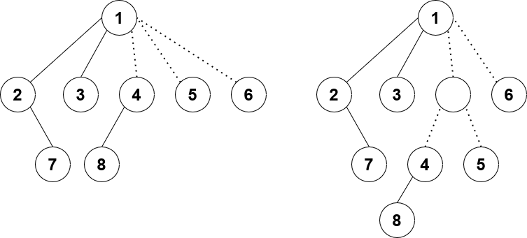
The solid lines represent preferred edges, and the dotted lines are unpreferred/virtual edges. The nodes 2, 7, 1, 3 form a preferred path in that order. Node 1 has both a left and right preferred child, and it has 3 virtual children.
The LCT on the left is what an ordinary LCT might look like. Node 1 has 3 virtual children, which is more than 2. Therefore, we binarize its virtual children by introducing a new fake vertex to connect both 4 and 5. Now as seen in the LCT on the right, each node has at most 2 preferred children and 2 virtual children (up to 4 children in total). So simple!
If only… the devil is in the details…
If you were to go and start coding this idea right now, you might realize there are quite few pitfalls to keep in mind while coding. The next few sections will be dedicated to talking about some of the implementation details in depth.
The Access Method
Since everything in LCTs revolve around access, let’s first characterize the access method. Here’s what a typical access method might look like:
1
2
3
4
5
6
7
8
9
10
11
12
13
14
15
16
17
18
19
20
21
22
23
24
25
26
27
28
29
30
31
// tr is a global array storing each of the LCT nodes
// p is the parent and ch is a size 4 array of its children
void attach(int u, int d, int v) {
    tr[u].ch[d] = v;
    tr[v].p = u;
    pull(u);
}

// adds v as a virtual child of u
void add(int u, int v) {
    tr[u].vir += tr[v].sum;
}

// removes v as a virtual child of u
void rem(int u, int v) {
    tr[u].vir -= tr[v].sum;
}

void access(int u) {
    splay(u);
    add(u, tr[u].ch[1]);        // the preferred path ends at u, so any node with greater depth should be disconnected and made virtual instead
    attach(u, 1, 0);            // sets the right preferred child of u to null (0)
    while (tr[u].p) {
        int v = tr[u].p;
        splay(v);
        add(v, tr[v].ch[1]);    // disconnect any node with greater depth than v, so result is a preferred path ending at v
        rem(v, u);              // u is no longer a virtual child of v
        attach(v, 1, u);        // u is now the right preferred child of v
        splay(u);
    }
}
You’ll be glad to hear this isn’t far from the final product. The fundamental process of accessing a node remains the same. The only difference is that the add and rem methods become more complex, because we may have to introduce more fake nodes for binarization.
The Add Method
Firstly, let’s take a look at add.
1
2
3
4
5
6
7
8
9
10
11
12
13
14
// attaches v as a virtual child of u
void add(int u, int v) {
    if (!v)
        return;
    for (int i=2; i<4; i++)
        if (!tr[u].ch[i]) {
            attach(u, i, v);
            return;
        }
    int w = newFakeNode();
    attach(w, 2, tr[u].ch[2]);
    attach(w, 3, v);
    attach(u, 2, w);
}
The first case is straightforward: if one of our 2 virtual children is null, simply set $v$ as that virtual child instead.
1
2
3
4
5
for (int i=2; i<4; i++)
    if (!tr[u].ch[i]) {
        attach(u, i, v);
        return;
    }
The second case is when $u$ already has 2 virtual children. In that case, we create a new fake node connecting both $v$ and one of our old virtual children, and substituting that as the new virtual child.
1
2
3
4
int w = newFakeNode();
attach(w, 2, tr[u].ch[2]);
attach(w, 3, v);
attach(u, 2, w);
The rem method is slightly more complex and requires the introduction of several other concepts first, so we’ll come back to that in a minute.
Bound on Fake Node Creation
Firstly, while we’re on the subject of fake nodes, how many fake nodes will we create? If we only create fake nodes without destroying, we could create as many as the number of preferred child changes, which is $\mathcal O(n \log n)$ with significant constant. That’s often an undesirable amount of memory to use. Fortunately, observe that at any point, we only need at most $n$ fake nodes to binarize the entire tree. Therefore, as long as we recycle memory and destroy fake nodes in the rem method when they become unnecessary, we will limit our memory usage to just $2n$ nodes.
Fake Nodes in Our Preferred Paths?
If we just splay willy-nilly in our access method, we might connect fake nodes into our preferred paths. This is undesirable because it becomes messy to keep track of where fake nodes are and when we can destroy them for preserving memory. Thus, we’ll need to make the following change to access.
Old Access
1
2
3
4
5
6
7
8
9
10
11
12
13
void access(int u) {
    splay(u);
    add(u, tr[u].ch[1]);
    attach(u, 1, 0);
    while (tr[u].p) {
        int v = tr[u].p;
        splay(v);
        add(v, tr[v].ch[1]);
        rem(v, u);
        attach(v, 1, u);
        splay(u);
    }
}
Instead of int v = tr[u].p, we will do int v = par(u), where par is a method giving us the lowest ancestor of $u$ that is not a fake node.
1
2
3
4
5
6
int par(int u) {
    int v = tr[u].p;
    while (tr[v].fake)
        v = tr[v].p;
    return v;
}
However, this is not good enough. There is no height guarantee on our binary tree formed from fake nodes, so we could be repeating $\mathcal O(n)$ work each time and break complexity. The solution? Make it a splay. So we have two splays: the usual one in ordinary LCT and one on the fake nodes. The new par method would thus look like the following:
1
2
3
4
5
6
7
int par(int u) {
    int v = tr[u].p;
    if (!tr[v].fake)
        return v;
    fakeSplay(v);
    return tr[v].p;
}
Technically...
So I said the old par method wasn’t ok because the height could be $\mathcal O(n)$, but when I copy pasted it into my code and submitted it, it still got AC. My guess is it’s very difficult to construct a sequence of operations to lead to a degenerate fake node binary tree, so in practice it still runs fast for random data? Either way, just use the second version to be safe.
Fake Splay
There’s no need to remake a new set of splay functions for the fake splay cause that’s wasteful. Instead, strive to write reusable splay code that works for both versions depending on a parameter passed in. I don’t want to get too into the weeds of the splay implementation because that’s more about splay trees and less about LCT, and because everyone implements splay differently, so I’ll just copy paste my before and after showing how I adapted splay tree code to work for both versions:
Before
1
2
3
4
5
6
7
8
9
10
11
12
13
14
15
16
17
18
19
20
21
22
23
24
25
26
27
28
29
30
31
32
33
34
void attach(int u, int d, int v) {
    tr[u].ch[d] = v;
    tr[v].p = u;
    pull(u);
}

int dir(int u) {
    int v = tr[u].p;
    return tr[v].ch[0] == u ? 0 : tr[v].ch[1] == u ? 1 : -1;
}

void rotate(int u) {
    int v = tr[u].p, w = tr[v].p, du = dir(u), dv = dir(v);
    attach(v, du, tr[u].ch[!du]);
    attach(u, !du, v);
    if (~dv)
        attach(w, dv, u);
    else
        tr[u].p = w;
}

void splay(int u) {
    push(u);
    while (~dir(u)) {
        int v = tr[u].p, w = tr[v].p;
        push(w);
        push(v);
        push(u);
        int du = dir(u), dv = dir(v);
        if (~dv)
            rotate(du == dv ? v : u);
        rotate(u);
    }
}
After
1
2
3
4
5
6
7
8
9
10
11
12
13
14
15
16
17
18
19
20
21
22
23
24
25
26
27
28
29
30
31
32
33
34
35
36
37
void attach(int u, int d, int v) {
    tr[u].ch[d] = v;
    tr[v].p = u;
    pull(u);
}

int dir(int u, int o) {
    int v = tr[u].p;
    return tr[v].ch[o] == u ? o : tr[v].ch[o+1] == u ? o + 1 : -1;
}

void rotate(int u, int o) {
    int v = tr[u].p, w = tr[v].p, du = dir(u, o), dv = dir(v, o);
    if (dv == -1 && o == 0)
        dv = dir(v, 2);
    attach(v, du, tr[u].ch[du^1]);
    attach(u, du ^ 1, v);
    if (~dv)
        attach(w, dv, u);
    else
        tr[u].p = w;
}

// call splay(u, 0) for ordinary and splay(u, 2) for fake
void splay(int u, int o) {
    push(u);
    while (~dir(u, o) && (o == 0 || tr[tr[u].p].fake)) {
        int v = tr[u].p, w = tr[v].p;
        push(w);
        push(v);
        push(u);
        int du = dir(u, o), dv = dir(v, o);
        if (~dv && (o == 0 || tr[w].fake))
            rotate(du == dv ? v : u, o);
        rotate(u, o);
    }
}
How to Do the Lazy Propagation
A first thought on doing lazy propagation is to simply maintain 2 lazy values: one for the path, and one for the subtree. However, it’s important to ensure the two lazy values cover a disjoint partition of nodes, because otherwise there’s no way to properly order the combination of lazy values affecting the intersection of the two partitions. To clarify what I mean, consider the range set operation applied to a simple array.
\[[1, 2, 3, 4, 5]\]Say we range set all values in the interval $[1, 3]$ to $7$, range set the interval $[3, 5]$ to $9$, and then range set the interval $[1, 3]$ again to $10$. Say we maintain two lazy values, one for the interval $[1, 3]$ and one for the interval $[3, 5]$, which would be $9$ and $10$ respectively. The issue is that it isn’t obvious what the lazy effect on index $3$ is. In this case, we could maintain the time stamp of both lazy values and use the later one to determine the effect, but you can see how if we use some other lazy operation where intermediate operations, not just the last one, have an effect (e.g. applying an affine function $x := ax + b$ to a range), then this breaks down.
The same applies for the LCT model. If a LCT node has two lazy values, one for the path and one for subtree (in the represented tree), then we need them to cover a disjoint partition of all nodes in the subtree (in the LCT, not in the represented tree). For brevity, let’s denote the first lazy value as plazy (short for “path lazy”) and the second value as slazy (short for “subtree lazy”). We will also define 3 aggregates in each node: path, sub, and all. path is the standard path aggregate used in ordinary LCT, so it is tr[tr[u].ch[0]].path + tr[tr[u].ch[1]].path + tr[u].val. sub will be everything else not covered in path, so tr[tr[u].ch[0]].sub + tr[tr[u].ch[1]].sub + tr[tr[u].ch[2]].all + tr[tr[u].ch[3]].all. And finally, all is just a combination of both to get everything in this LCT subtree, or tr[u].all = tr[u].path + tr[u].sub. Putting it all together, we get the following pull method for recalculating the aggregates in a node:
1
2
3
4
5
6
void pull(int u) {
    if (!tr[u].fake)
        tr[u].path = tr[tr[u].ch[0]].path + tr[tr[u].ch[1]].path + tr[u].val;
    tr[u].sub = tr[tr[u].ch[0]].sub + tr[tr[u].ch[1]].sub + tr[tr[u].ch[2]].all + tr[tr[u].ch[3]].all;
    tr[u].all = tr[u].path + tr[u].sub;
}
Now for pushing down the lazy tags! Pushing plazy is the same as ordinary LCT: push down to the 0th and 1st child. Pushing slazy is slightly less obvious. Specifically, we will only update slazy for the 0th and 1st child, and we will update both plazy and slazy for the 2nd and 3rd child. For the 2nd and 3rd child, we update both lazy values because all values in that LCT subtree represent nodes affected in the real subtree, so both path and sub must be updated. But why don’t we update both lazy values in the 0th and 1st child? It’s because if we were to receive an update for this entire subtree from the parent, then there are 2 cases:
- The current node is a preferred child of its parent. In this case, recursively go up until we hit case 2.
- The current node is a virtual child of its parent. In this case, when we push down from the parent, the current node would have gotten both its
plazyandslazyvalues updated. So thepathpart of its LCT subtree is already fully updated. If we were to updateplazyof its 0th and 1st children again when pushing down from the current node, then we would be applying the update twice to the path.
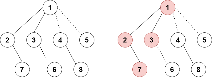
Say node 1 is following case 2, meaning it is a virtual child of its parent. Node 1 just received a tag pushed down from its parent, so its plazy and slazy values are updated. The nodes highlighted in red are the ones already correctly accounted for by plazy. If we were to push down and update node 2’s plazy with node 1’s slazy as well, then node 2 would be receiving the update twice which is incorrect.
So putting everything together gives us the following push method:
1
2
3
4
5
6
7
8
9
10
11
12
13
14
15
16
17
18
19
20
21
22
23
24
25
26
27
28
29
30
31
32
33
34
35
36
void pushPath(int u, const Lazy &lazy) {
    if (!u || tr[u].fake)
        return;
    tr[u].val += lazy;
    tr[u].path += lazy;
    tr[u].all = tr[u].path + tr[u].sub;
    tr[u].plazy += lazy;
}

void pushSub(int u, bool o, const Lazy &lazy) {
    if (!u)
        return;
    tr[u].sub += lazy;
    tr[u].slazy += lazy;
    if (!tr[u].fake && o)
        pushPath(u, lazy);
    else
        tr[u].all = tr[u].path + tr[u].sub;
}

void push(int u) {
    if (!u)
        return;
    if (tr[u].plazy.lazy()) {
        pushPath(tr[u].ch[0], tr[u].plazy);
        pushPath(tr[u].ch[1], tr[u].plazy);
        tr[u].plazy = Lazy();   // empty constructor for lazy resets it
    }
    if (tr[u].slazy.lazy()) {
        pushSub(tr[u].ch[0], false, tr[u].slazy);
        pushSub(tr[u].ch[1], false, tr[u].slazy);
        pushSub(tr[u].ch[2], true, tr[u].slazy);
        pushSub(tr[u].ch[3], true, tr[u].slazy);
        tr[u].slazy = Lazy();
    }
}
Note
This code uses a style of lazy where the values are correctly updated at the same time that the node receives the tag. I usually implement lazy in a different style, where the values are correctly updated when the node pushes down its tag, but I found implementing lazy propagation the first way yields a much better constant factor.
The Rem Method
I promised you we would come back to the rem method. Well, we’re finally ready to tackle it!
1
2
3
4
5
6
7
8
9
10
11
12
13
14
15
16
17
18
19
20
21
22
23
24
25
int dir(int u, int o) {
    int v = tr[u].p;
    return tr[v].ch[o] == u ? o : tr[v].ch[o+1] == u ? o + 1 : -1;
}

void recPush(int u) {
    if (tr[u].fake)
        recPush(tr[u].p);
    push(u);
}

void rem(int u) {
    int v = tr[u].p;
    recPush(v);
    if (tr[v].fake) {
        int w = tr[v].p;
        attach(w, dir(v, 2), tr[v].ch[dir(u, 2) ^ 1]);
        if (tr[w].fake)
            splay(w, 2);    // fake splay
        free(v);
    } else {
        attach(v, dir(u, 2), 0);
    }
    tr[u].p = 0;
}
What’s happening here? Let’s break it down. $u$ is the node that we are disconnecting from its parent, $v$. First consider the easier of the two cases:
1
2
3
} else {
    attach(v, dir(u, 2), 0);
}
This clause triggers when $v$ is not a fake node. In this case, it’s exactly the same as ordinary LCT. Remove $u$ as a virtual child of $v$.
We could handle the second case in the same way, but there’s an extra consideration. If $v$ is fake, then after removing $u$, $v$ only has one virtual child and is therefore obsolete. We can destroy the node and attach $v$’s other child directly to $v$’s parent instead! This step is necessary to ensure our number of fake nodes remains under our bound of $n$.
There’s one more consideration: correct application of pushes and pulls. Consider the following scenario:

We are calling rem on node 4 and attaching it as a preferred child of 1 instead. The red fake node has a pending lazy tag waiting to be pushed down. The left and right diagrams show before and after the procedure.
See the issue? When we remove $u$ and reattach it above, it could “dodge” a lazy tag that it’s supposed to receive. So to remedy this, we need to call push on all fake ancestors of $u$ up to the next non-fake node, which is what the method recPush does in my code. Finally, notice that after removing $u$, we would need to call pull again on all fake ancestors up to the next non-fake node to correctly set their values. We could create another method recPull with similar structure to recPush. Or, we could just call splay at the end to correctly set all the node values moving up. Calling splay would also fix any amortized complexity concerns from calling recPush.
And that’s it! We’ve successfully implemented our new version of access!
The Rest of the Methods
Once you have access, every other method is sincerely trivial. I’ll include them here for sake of completeness.
Reroot, link, cut, lca, and path query/update are all completely identical to ordinary LCT.
Recap of Those Methods
reroot(u):
- Introduce a lazy flip tag that swaps the 0th and 1st child of a node
- Access $u$
- Apply lazy flip tag to $u$
link(u, v):
- Reroot $u$
- Access $v$
- Call
add(v, u)
cut(u, v):
- Reroot $u$
- Access $v$
- Disconnect $v$’s 0th child
- Pull $v$
lca(u, v):
- Modify the access method to return the last parent of $u$ in the while loop before it becomes the root
- Access $u$
- Return access $v$
path(u, v):
- Reroot $u$
- Access $v$
- Return $v$’s
path/update $v$’splazy
Finally, for subtree queries/updates. Say we are querying for the subtree of $u$ given that $r$ is the root. First:
- Reroot $r$
- Access $u$
Now, $u$’s subtree in the represented tree consists of all the virtual subtrees hanging off of $u$, plus $u$ itself. So in other words, tr[tr[u].ch[2]].all + tr[tr[u].ch[3]].all + tr[u].val. For query, we just return that value. For update, we update tr[u].val directly, and then we update both the plazy and slazy values of its two virtual children. We do not touch the 0th or 1st child, since those are not part of $u$’s subtree.
The Code
I’ve pasted snippets here and there, but if you’re still fuzzy on some of the implementation details, you can see my complete code here.
Performance
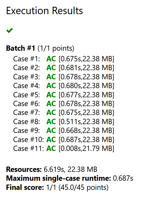
Presumably, the complexity of this augmentation of LCT is still $\mathcal O(\log n)$, but with a significant constant factor (this article estimates the constant factor to be $97$). On DMOJ, it runs in around 0.6-0.7 seconds for $n, q \leq 10^5$. On Library Checker, it runs in a little over 1 second for $n, q \leq 2 \cdot 10^5$. So its performance is closer to $\mathcal O(\log^2 n)$ in practice. Some of the implementations in the Chinese articles run faster than mine, but that seems to come at the cost of readability and some strange code, and my implementation is fast enough for almost all reasonable competitive programming purposes.
Applications