Applications of Divide and Conquer
Divide and conquer (D&Q for short) is a common and powerful problem solving paradigm in the world of algorithms. There are numerous well-known examples such as merge sort and fast Fourier transform, and in this article I will cover some (maybe less common) applications of D&Q that are more specific to competitive programming. The sections progress from simple to complex, so more experienced competitors can skip to a later section of the article.
Core Concept
The core concept of D&Q is to divide our problem into subproblems, then combine them together in some way. Consider the classic example of merge sort, a D&Q algorithm to sort an array. Let’s write a recursive function sort(a) which will sort the array $a$. First, we can split our array into two halves and sort each of those halves recursively with sort(left) and sort(right):
1
2
3
4
5
6
7
8
9
10
11
12
13
14
15
void sort(vector<int> &a) {
    int n = (int) a.size();
    if (n == 1)
        return;
    int m = n / 2;
    // two halves denoted "left" and "right"
    vector<int> left, right;
    for (int i=0; i<m; i++)
        left.push_back(a[i]);
    for (int i=m; i<n; i++)
        right.push_back(a[i]);
    sort(left);
    sort(right);
    // now we need to combine the result of the two halves in some way
}
Then, after we’ve sorted the two individual halves, we can merge them together in linear time with the following algorithm:
1
2
3
4
5
6
7
8
9
// merges two sorted arrays into one sorted array
int n = (int) left.size(), m = (int) right.size(), i = 0, j = 0;
vector<int> comb;
while (i < n || j < m) {
    if (i < n && (j == m || left[i] < right[j]))
        comb.push_back(left[i++]);
    else
        comb.push_back(right[j++]);
}
Complete Mergesort Code
1
2
3
4
5
6
7
8
9
10
11
12
13
14
15
16
17
18
19
20
21
22
23
24
25
26
vector<int> merge(const vector<int> &left, const vector<int> &right) {
    int n = (int) left.size(), m = (int) right.size(), i = 0, j = 0;
    vector<int> comb;
    while (i < n || j < m) {
        if (i < n && (j == m || left[i] < right[j]))
            comb.push_back(left[i++]);
        else
            comb.push_back(right[j++]);
    }
    return comb;
}

void sort(vector<int> &a) {
    int n = (int) a.size();
    if (n == 1)
        return;
    int m = n / 2;
    vector<int> left, right;
    for (int i=0; i<m; i++)
        left.push_back(a[i]);
    for (int i=m; i<n; i++)
        right.push_back(a[i]);
    sort(left);
    sort(right);
    a = merge(left, right);
}
In general, the code for any divide and conquer algorithm might look something like this:
1
2
3
4
5
solve(whole part) {
    solve(left part)
    solve(right part)
    combine(result of solve(left part), result of solve(right part))
}
Analyzing the time complexity of a D&Q algorithm isn’t always obvious, and the most common way it’s done in literature is using the master theorem. However, I personally don’t find the master theorem very intuitive, so I prefer to just analyze the complexity by looking at the recursive tree of states. To explain what I mean, take a look at the following diagram for merge sort:
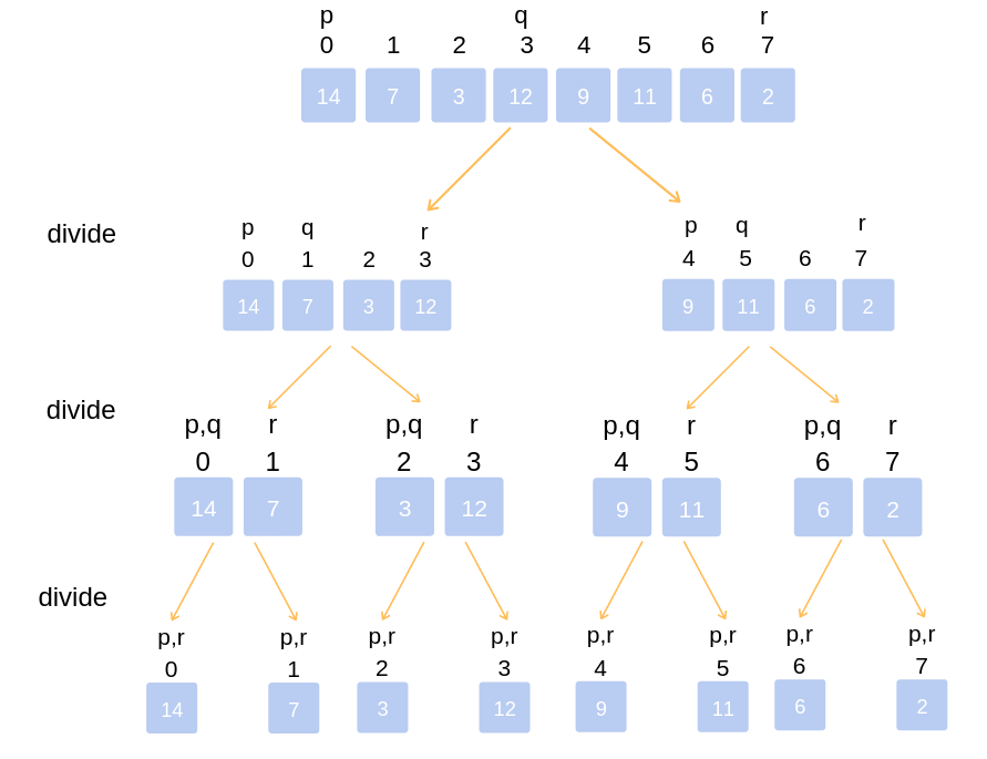
To understand the complexity of merge sort, we note that the height of the recursive tree is at most $\mathcal O(\log n)$, because on each layer the size of the subarrays we are working with get halved, and we can only half an array of size $n$ at most $\log_2 n$ times. On each layer, we are merging together two subarrays from the next layer, and the sum of all subarray sizes is the size of the original array, or $n$. Since we do $\mathcal O(n)$ work on each of $\mathcal O(\log n)$ layers, the complexity of merge sort is $\mathcal O(n \log n)$.
This was a traditional simple example, so now let’s jump into some harder problems!
Codeforces Edu 94E: Clear the Multiset
The problem essentially translates to the following: given an array, we can perform two types of operations:
- Subtract 1 from some subarray of non-zero values.
- Subtract any positive $x$ from any one value.
What is the minimum number of operations to reduce the array to all 0s?
There is an approach to this problem using dynamic programming, but let’s consider a D&Q approach. Let’s denote solve(l, r) as the minimum number of operations to reduce the subarray $a[l, r]$ to 0. For now, assume $a_i > 0$. An upper bound on our answer is r - l + 1 by applying the type 2 operation to reduce each array element to 0. Now what if we want to perform type 1 operations? Note that it’s always optimal to apply type 1 operations to the entire subarray, because that gets us closer to reducing all of them to 0. It is never optimal to use type 1 operations on some subset of the subarray, then type 2 operations in between, because we can achieve the same effect by applying type 1 operations to the entire array when possible and use less operations. We can apply type 1 operations until some element gets reduced to 0, which will first be the minimum element. After some index $a_m$ gets reduced to 0, we can compute and add solve(l, m - 1) and solve(m + 1, r) as subproblems. The code looks as follows:
1
2
3
4
5
6
7
8
9
10
11
12
13
14
int solve(int l, int r) {
    if (l > r)
        return 0;
    // we will apply type 1 operation (min a_i) times
    int mn = *min_element(a.begin() + l, a.begin() + r + 1), idx = -1;
    for (int i=l; i<=r; i++) {
        a[i] -= mn;
        if (a[i] == 0)
            idx = i;    // split at the index that drops to 0 (notice that ties don't matter)
    }
    assert(idx != -1);
    // return minimum of our two options: solve recursively, or just apply type 2 operations to each element
    return min(solve(l, idx - 1) + solve(idx + 1, r) + mn, r - l + 1);
}
An Aside
Notice that this code allows applying type 2 operations on some $a_i = 0$, which is technically not allowed. Luckily, we will never do that in the optimal solution anyways, so it’s ok that our code permits this possibility. This is actually a very common trick in CP: relaxing the conditions of the problem to ease the implementation because we know the optimal solution will follow a stricter set of conditions. This problem is another example of that trick (though it’s not a D&Q problem).
One question left: what’s the time complexity? One way of bounding the time complexity is doing the same thing we did in our merge sort example: bound the height of the recursive tree and the amount of work we perform on each height. The worst case would be doing uneven splits every time (i.e. always having the minimum element be $l$): $[1, n] \implies [2, n] \implies [3, n] \implies \dots$, giving us $\mathcal O(n)$ height. On each layer, we iterate over all the elements in the array at most once in one of the states on that layer, giving us $\mathcal O(n)$ work per layer, so our complexity is $\mathcal O(n^2)$, which is fast enough for the constraints of this problem.
Another approach is simply counting the number of total states. A naive bound would be $\mathcal O(n^2)$ states, since there are $\frac{n(n+1)}{2}$ possible subarrays, but we can prove a better bound. Consider this crudely drawn recursive tree:
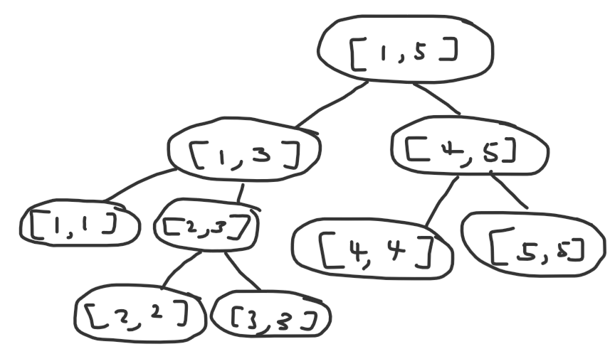
A circle with some $[l, r]$ written on it represents the recursive state solve(l, r).
In this diagram, I actually include the minimum index still, so instead of splitting $[l, r]$ into $[l, m - 1]$ and $[m + 1, r]$, I split it into $[l, m]$ and $[m + 1, r]$. I do this because this is a general proof that extends to other problems, and including $m$ in one of the intervals can only make the complexity worse, so the proof still applies to this problem.
Now here’s the intuition: let’s pretend indices $1, 2, \dots, n$ actually refer to nodes in a graph. The state $[l, r]$ refers to a connected component of vertices $l, l + 1, \dots, r$. And initially, we have $[1, n]$ representing a line graph with edges connecting $(i, i + 1)$ for all $1 \leq i < n$, or $n - 1$ total edges. What does a split of a state into two other states represent in this analogy? It represents deleting some edge $(m, m + 1)$ and splitting the component into two separate ones. And since we can only delete at most $n - 1$ edges, we only have at most $2(n - 1) + 1$ states, or $\mathcal O(n)$ states! A naive bound on the amount of work we do at each state is $\mathcal O(n)$, so the complexity is $\mathcal O(n^2)$.
Notice that our second way of analyzing the complexity more easily lends itself to a subquadratic solution. Instead of naively iterating to find the minimum index, we can use a RMQ sparse table to instantly find it in $\mathcal O(1)$. And instead of subtracting mn from each index like in the code above, we notice that we’re simply subtracting mn from every array element, so we can instead maintain some extra parameter delta in our recursive method to keep track of how much we’ve subtracted from all elements in our current range. So we’ve now reduced the amount of work done at each state to $\mathcal O(1)$, giving us an $\mathcal O(n)$ or $\mathcal O(n \log n)$, depending on how we precompute our sparse table.
$\mathcal O(n)$ Code
1
2
3
4
5
6
7
8
int solve(int l, int r, int delta) {
    if (l > r)
        return 0;
    // we will apply type 1 operation (min a_i) times
    int idx = sparse_table.query(l, r), mn = a[idx] - delta;
    // return minimum of our two options: solve recursively, or just apply type 2 operations to each element
    return min(solve(l, idx - 1, delta + mn) + solve(idx + 1, r, delta + mn) + mn, r - l + 1);
}
An Aside
If you're familiar with top-down dynamic programming, you may recognize the similarities in code. You could think of this D&Q strategy as a special case of dynamic programming, except we don't need to memoize because our recursive structure is a tree, so each state is visited exactly once. If we were to draw a "recursive tree of states" for a typical dynamic programming problem, it would likely not be a tree, but be a DAG instead, so we would need memoization.binarysearch.com: Every Sublist Containing Unique Element
I find this problem unusually hard for a coding interview question, especially one of “medium” difficulty, but I digress.
We’ll deploy a similar approach to the previous problem. Let solve(l, r) return true if every subarray contains a unique element, and false otherwise. Right off the bat, if $a[l, r]$ contains no unique element, then we are done and can return false. Otherwise, let’s say $a_m$ is a unique element. Any subarray of $a[l, r]$ containing $a_m$ will for sure contain a unique element, which would be $a_m$, so a subarray of $a[l, r]$ containing no unique elements must not contain $a_m$. Thus, to search for the existence of such a subarray, we split into two subproblems solve(l, m - 1) and solve(m + 1, r), and if any of those return false, we also return false from solve(l, r). To check if there is a unique element, we can iterate over all elements and store them in a hashmap. The worst case complexity of this algorithm is $\mathcal O(n^2)$, since we visit $\mathcal O(n)$ states and perform $\mathcal O(n)$ work at each state.
We can apply a simple optimization: instead of splitting just at one index, we can split at every unique index. That is, if $a_{m_1}, a_{m_2}, \dots, a_{m_k}$ are all unique elements, then we can split solve(l, r) into solve(l, a[m_1] - 1), solve(a[m_1] + 1, a[m_2] - 1), …, solve(a[m_k] + 1, r). While the worst case complexity is still $\mathcal O(n^2)$, this optimization is sufficient to get AC on this problem. Weak test cases I guess.
Optimized $\mathcal O(n^2)$
1
2
3
4
5
6
7
8
9
10
11
12
13
14
15
16
17
18
19
20
21
bool recur(int l, int r, const vector<int> &nums) {
    if (l >= r)
        return true;
    unordered_map<int, int> mp;
    for (int i=l; i<=r; i++)
        mp[nums[i]]++;
    int last = l;
    bool uniq = false;
    for (int i=l; i<=r; i++)
        if (mp[nums[i]] == 1) {
            uniq = true;
            if (!recur(last, i - 1, nums))
                return false;
            last = i + 1;
        }
    return uniq && recur(last, r, nums);
}

bool solve(vector<int>& nums) {
    return recur(0, (int) nums.size() - 1, nums);
}
The above code ACs in 235 ms.
But we can do better. We can achieve worst case $\mathcal O(n \log n)$. To do that, we apply the following optimization: instead of always iterating our for loop from the left to right, we iterate from both sides. So for the subarray $a[l, r]$, we first check $a_l$, then $a_r$, then $a_{l+1}$, then $a_{r-1}$, then $a_{l+2}$, and so on. We can check if some $a_m$ is unique in $a[l, r]$ in $\mathcal O(1)$ by precomputing left[m] and right[m], arrays storing the index of the next occurrence of $a_m$ to the left or right of $a_m$. So if a state splits into two states of size $a$ and $b$, the amount of work done at that state is $\mathcal O(\min(a, b))$.
It turns out this single optimization is sufficient to achieve $\mathcal O(n \log n)$. To understand why, let’s once again consult the recursive tree of states.
Once again, we use the analogy of nodes and components that we used in the previous problem (treating each state representing the range $[l, r]$ as a component of nodes $l, l + 1, \dots, r$). Instead of thinking of it as splitting a graph into individual nodes, let’s think in reverse: we have $n$ nodes, and want to merge them into one component. Two child states merge to become one state. If we merge two components of size $a$ and $b$, we do $\min(a, b)$ work. Does this sound familiar? That’s right, this is just small-to-large merging! In small-to-large merging, when we merge two components of size $a$ and $b$, we only iterate over the nodes in the smaller of the two components, so we do $\mathcal O(\min(a, b))$ work. That’s essentially the same thing we’re doing here: we only do $\mathcal O(\min(a, b))$ work since we only iterate as much as twice the size of the smaller subproblem in our divide and conquer (twice since we iterate on both ends). And so by the same analysis as small-to-large merging, our runtime is $\mathcal O(n \log n)$.
Small-to-Large Complexity Proof
Consider merging two components $A$ and $B$, with sizes $|A|$ and $|B|$. WLOG, assume $|A| \leq |B|$. Small-to-large merging will iterate over each node in $A$ and add it to $B$, doing $\mathcal O(|A|)$ work. Let’s track how many times we iterate over a node. If a node gets iterated over, it means it was in the smaller of two components being merged together. So after the merging, it will be in a component that is at least twice the size of its original component. The size of a component can only be doubled $\mathcal O(\log n)$ times before it reachs size $n$. So a node can only be iterated over at most $\mathcal O(\log n)$ times. Thus, when we sum up the work done on each of $n$ nodes, we get $\mathcal O(n \log n)$ complexity.
HackerRank: Find the Path
A naive solution is to run Dijkstra for each query, giving us a $\mathcal O(nmq \log (nm))$ approach. It’s difficult to improve upon this online algorithm with some sort of precomputation, because the optimal path could go “backwards” or wrap around in any arbitrary snake-like path. So as you might have guessed, we’ll solve this problem offline with D&Q on the queries.
Let’s consider some recursive function solve(l, r) that will process queries for which the path between its endpoints lies in columns $[l, r]$. Consider column $m = \lfloor \frac{l + r}{2} \rfloor$. Any path in columns $[l, r]$ falls into one of three cases:
- The path lies solely in columns $[l, m]$.
- The path lies solely in columns $[m + 1, r]$.
- The path exists in both halves and crosses over column $m$ (note that both endpoints can still be in the same half for this case).
Cases 1 and 2 will be handled in our recursive subproblems, solve(l, m) and solve(m + 1, r). For case 3, notice that since our path crosses column $m$, it can be expressed as the concatenation of two paths originating from a single cell in column $m$. Since $n$ is small, we can brute force each cell in column $m$ and run Dijkstra from that cell, and update our answer for all queries with endpoints in columns $[l, r]$. We have a $\mathcal O(\log m)$ height recursive tree with $\mathcal O(n(nm \log (nm) + q))$ work on each layer, giving us $\mathcal O(n \log m (nm \log (nm) + q))$ as our final complexity.
Old Messy Code Written 4 Months Ago
1
2
3
4
5
6
7
8
9
10
11
12
13
14
15
16
17
18
19
20
21
22
23
24
25
26
27
28
29
30
31
32
33
34
35
36
37
38
39
40
41
42
43
44
45
46
47
48
49
50
51
52
53
54
55
56
57
58
59
60
61
62
63
64
65
66
67
68
69
70
71
72
73
74
75
76
77
#include <bits/stdc++.h>
using namespace std;

const int INF = 1e9;

const int dx[] = {-1, 0, 1, 0};
const int dy[] = {0, 1, 0, -1};

typedef tuple<int, int, int> node;

int main() {
    ios_base::sync_with_stdio(false);
    cin.tie(NULL);

    int n, m;
    cin >> n >> m;
    vector<vector<int>> a(n, vector<int>(m));
    for (int i=0; i<n; i++)
        for (int j=0; j<m; j++)
            cin >> a[i][j];
    int q;
    cin >> q;
    vector<array<int, 5>> queries;
    for (int i=0; i<q; i++) {
        int r1, c1, r2, c2;
        cin >> r1 >> c1 >> r2 >> c2;
        queries.push_back({r1, c1, r2, c2, i});
    }

    vector<vector<vector<int>>> dist(n, vector<vector<int>>(n, vector<int>(m)));

    auto dijkstra = [&] (int s, int t, int l, int r) -> void {
        for (int i=0; i<n; i++)
            for (int j=l; j<=r; j++)
                dist[s][i][j] = INF;
        priority_queue<node, vector<node>, greater<node>> pq;
        pq.emplace(dist[s][s][t] = a[s][t], s, t);
        while (!pq.empty()) {
            auto [d, x, y] = pq.top();
            pq.pop();
            if (d > dist[s][x][y])
                continue;
            for (int i=0; i<4; i++) {
                int nx = x + dx[i], ny = y + dy[i];
                if (0 <= nx && nx < n && l <= ny && ny <= r && d + a[nx][ny] < dist[s][nx][ny])
                    pq.emplace(dist[s][nx][ny] = d + a[nx][ny], nx, ny);
            }
        }
    };

    vector<int> ret(q, INF);

    auto solve = [&] (auto &self, int l, int r, const vector<array<int, 5>> &queries) -> void {
        if (l > r)
            return;
        int x = (l + r) / 2;
        for (int i=0; i<n; i++)
            dijkstra(i, x, l, r);
        vector<array<int, 5>> left, right;
        for (auto [r1, c1, r2, c2, i] : queries) {
            for (int j=0; j<n; j++)
                ret[i] = min(ret[i], dist[j][r1][c1] + dist[j][r2][c2] - a[j][x]);
            if (c1 < x && c2 < x)
                left.push_back({r1, c1, r2, c2, i});
            else if (c1 > x && c2 > x)
                right.push_back({r1, c1, r2, c2, i});
        }
        self(self, l, x - 1, left);
        self(self, x + 1, r, right);
    };

    solve(solve, 0, m - 1, queries);
    for (int x : ret)
        cout << x << "\n";

    return 0;
}
CodeChef SEGPROD: Product on the Segment by Modulo
This problem is very peculiar because of its abnormally large bounds and weird input method to facilitate that. Let’s use the same approach as the previous problem, which is to D&Q on the queries. If our recursive method is currently processing the range $[l, r]$, then we can process all queries with the left endpoint $\leq m = \lfloor \frac{l + r}{2} \rfloor$ and right endpoint $> m$. To do this, we precompute $product[i, m]$ for all $l \leq i \leq m$ and $product[m + 1, i]$ for all $m < i \leq r$, and then each query is just the product of two precomputed values. Unfortunately, there are two issues with this approach:
- The problem forces us to solve it online, and this is an offline algorithm.
- The complexity is $\mathcal O((n + q) \log n)$, which is actually too much because $q \leq 2 \cdot 10^7$.
First, we can easily make our above algorithm online by storing all the prefix and suffix products precomputed at each layer, consuming $\mathcal O(n \log n)$ memory. Then, for each query, we can traverse recursively until we reach the correct layer, giving us $\mathcal O(\log n)$ per query.
Next, to improve our query complexity, we’ll use the following trick. Let’s round $n$ up to the nearest power of 2. Now take a look at the ranges we get in our recursive tree:
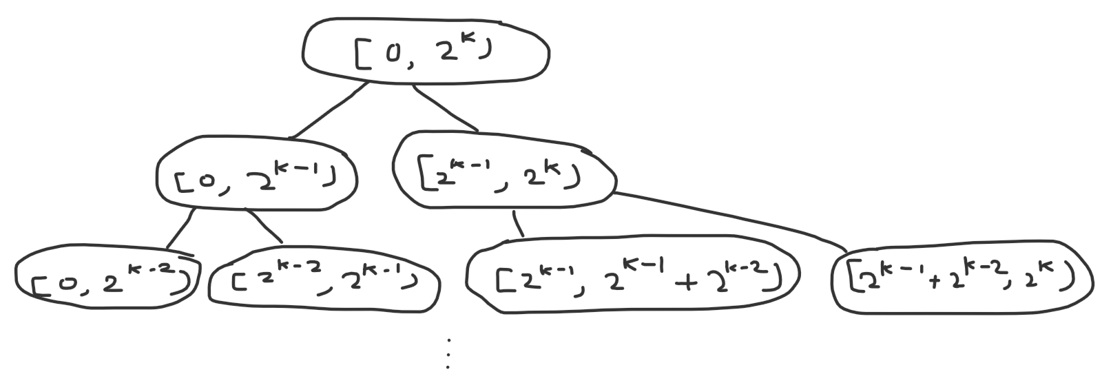
Notice anything peculiar? That’s right, each state splits into two deeper states based on whether a bit is on or off. So to find the correct layer where the left and right endpoint of our query lie on different sides of $m$, we simply need to find the most significant bit where they differ. Or in other words, we need to find the most significant bit in the xor of the endpoints, which can be computed in $\mathcal O(1)$ using builtin functions like __lg or precomputing a lookup table. So we’ve reduced our complexity to $\mathcal O(n \log n + q)$, which is fast enough to get AC.
Code
1
2
3
4
5
6
7
8
9
10
11
12
13
14
15
16
17
18
19
20
21
22
23
24
25
26
27
28
29
30
31
32
33
34
35
36
37
38
39
40
41
42
43
44
45
46
47
48
49
50
51
52
53
54
55
56
57
58
59
60
61
#include <bits/stdc++.h>
using namespace std;

int main() {
    ios_base::sync_with_stdio(false);
    cin.tie(NULL);

    int t;
    cin >> t;
    while (t--) {
        int n, p, q;
        cin >> n >> p >> q;
        int k = n == 1 ? 0 : __lg(n - 1) + 1;
        vector<int> a(1 << k);
        for (int i=0; i<n; i++)
            cin >> a[i];
        vector<int> b(q / 64 + 2);
        for (int &x : b)
            cin >> x;

        vector<vector<long long>> prod(k, vector<long long>(1 << k));

        auto recur = [&] (auto &self, int lg, int l, int r) -> void {
            if (lg < 0)
                return;
            int m = (l + r) / 2;
            for (int i=m-1; i>=l; i--)
                prod[lg][i] = a[i] * (i == m - 1 ? 1 : prod[lg][i+1]) % p;
            for (int i=m; i<r; i++)
                prod[lg][i] = a[i] * (i == m ? 1 : prod[lg][i-1]) % p;
            self(self, lg - 1, l, m);
            self(self, lg - 1, m, r);
        };

        auto query = [&] (int l, int r) -> int {
            if (l == r)
                return a[l];
            int lg = __lg(l ^ r);
            return prod[lg][l] * prod[lg][r] % p;
        };

        recur(recur, k - 1, 0, 1 << k);

        int x = 0, l, r;
        for (int i=0; i<q; i++) {
            if (i % 64 == 0) {
                l = (b[i / 64] + x) % n;
                r = (b[i / 64 + 1] + x) % n;
            } else {
                l = (l + x) % n;
                r = (r + x) % n;
            }
            if (l > r)
                swap(l, r);
            x = (query(l, r) + 1) % p;
        }
        cout << x << "\n";
    }

    return 0;
}
CDQ Divide and Conquer
This final section refers to a specific application of D&Q: CDQ D&Q, which I first read about in this Codeforces comment and in the linked PDF. The general gist of the technique is as follows: say we have a data structure and two types of operations:
- Update the data structure.
- Query for some aggregate in the data structure.
Additionally, say this problem is much easier to solve offline than online. That is, if all the update operations came before all the query operations, then there exists some offline algorithm to solve it. CDQ D&Q allows us to solve the online version with an extra $\mathcal O(\log n)$ factor.
For our example problem, we’ll use the one mentioned in this blog. There is an online solution using 2D segment tree that solves this in $\mathcal O(q \log^2 q)$, but 2D segment tree has a non-trivial time and memory constant factor and is often difficult to squeeze into the problem bounds if not intended.
How do we solve this problem offline? This is a well-known problem: we perform a linesweep. Every time we encounter the right endpoint of an interval, we insert the length of that interval at the left endpoint of that interval in a segment tree. Every time we encounter the right endpoint of some query, we query for the maximum value in $[l, r]$ in the segment tree.
Now for the CDQ D&Q step: we will perform divide and conquer on the time of each operation (first operation is at time 1, second operation at time 2, etc.). When we are considering all operations with time in the range $[l, r]$, we will do the following: consider $m = \lfloor \frac{l + r}{2} \rfloor$. For all update operations with time $\leq m$, we insert them. For all query operations with time $> m$, we apply the offline algorithm to update their answers. In this case, we are considering the contribution of all update operations in $[l, m]$ to the query operations in $[m + 1, r]$. Any update contributions in $[1, l - 1]$ would have been considered on an earlier layer, and any update contributions in $[m + 1, r]$ will be considered in a later layer, when we recurse to $[m + 1, r]$. The code would look something like the following:
1
2
3
4
5
6
7
8
9
10
11
12
13
void solve(int l, int r) {
    if (l == r)
        return;
    int m = (l + r) / 2;
    solve(l, m);
    vector<Op> updates, queries;
    for (int i=l; i<=m; i++)
        updates.push_back(op[i]);
    for (int i=m+1; i<=r; i++)
        queries.push_back(op[i]);
    offlineAlgorithm(updates, queries);
    solve(m + 1, r);
}
You might be wondering, why am I calling solve(l, m) before computing the contribution of $[l, m]$ on $[m + 1, r]$, and not after? In this problem, it doesn’t matter, but CDQ D&Q can also be applied to some dynamic programming problems where the order does matter. We would first call solve(l, m) to fully compute the final values of $dp[l, m]$. Once those DP values are final, we can rely on them to update the values $dp[m + 1, r]$. An example of this is in this Atcoder problem.
Finale
Hopefully you gleaned something from this tutorial! I tried to order the article from simplest to most complicated techniques, and tried to explain stuff unambiguously but also concisely. If you have any feedback or questions, don’t hesitate to drop a comment.
Problems (Roughly Ordered Based on Techniques Used in Article)
Codeforces Round 689D: Divide and Summarize
Codeforces Edu 105D: Dogeforces
Codeforces Round 429D: Destiny
SPOJ ADACABAA: Ada and Species
This is a very short list, so comment any other problems you know.
References (For CDQ D&Q)