Trivialize Linear Recurrence Problems with Berlekamp-Massey!
Berlekamp-Massey is a powerful tool that can knock out almost all linear recurrence problems, but it’s often explained in the context of BCH decoding in many online tutorials, making it difficult to understand in a more general sense. There’s TLE’s Codeforces blog, which contains all the core concepts of the algorithm but is a bit terse in my opinion. There’s also Massey’s paper, which is more on the mathematically rigorous side, and I have incorporated some of Massey’s proofs into the proof section of this article. The goal of this article is to explain Berlekamp-Massey using my intuition/understanding of it.
I promise this article isn’t hard, just dense. You won’t need an understanding of mathematics beyond high school, but it’s very easy to get lost if you don’t read line-by-line and just skim it. I tried my best to make it as clear as possible, but there’s only so much I can convey with words.
Table of Contents
- Definition of a Linear Recurrence
- Finding the $k$th Term of a Linear Recurrence
- What is the Berlekamp-Massey algorithm?
- An Example
- How does our process for choosing $d$ work?
- Which $b$ do we choose?
- The First Step
- Putting it all together in code…
- Test for Understanding
- Proofs
- Applications in Problems
- Problems
- References
Definition of a Linear Recurrence
Let’s say we have some arbitrary sequence of numbers:
\[\{1, 2, 4, 8, 13\}\]Now, let’s say we use the following rule to generate an infinite sequence from this initial sequence:
\[s_i = s_{i-1} + 2s_{i-2} + 5s_{i-3} - 3s_{i-4} - s_{i-5} \\ s_0 = 1 \\ s_1 = 2 \\ s_2 = 4 \\ s_3 = 8 \\ s_4 = 13\]Using this rule, what will the next element of this sequence be? What will $s_5$ be?
\[\begin{align*} s_5 &= s_4 + 2s_3 + 5s_2 - 3s_1 - s_0 \\ &= 13 + 2 \cdot 8 + 5 \cdot 4 - 3 \cdot 2 - 1 \\ &= 42 \end{align*}\]And what will $s_6$ be?
\[\begin{align*} s_6 &= s_5 + 2s_4 + 5s_3 - 3s_2 - s_1 \\ &= 42 + 2 \cdot 13 + 5 \cdot 8 - 3 \cdot 4 - 2 \\ &= 94 \end{align*}\]Following this rule, here are the first 10 elements of our sequence:
\[\{1, 2, 4, 8, 13, 42, 94, 215, 566, 1327, \dots\}\]We say the following sequence is defined by the linear recurrence $s_i = s_{i-1} + 2s_{i-2} + 5s_{i-3} - 3s_{i-4} - s_{i-5}$. The first 5 terms, $s_0, s_1, \dots, s_4$, are the base case or initial conditions of the recurrence. In general, a linear recurrence is a recurrence relation of the form:
\[s_i = \sum_{j=1}^n c_j s_{i-j}\]where $c_j$ are constants, and $n$ is the length of the linear recurrence. Technically, what we defined above is a homogeneous linear recurrence. A linear recurrence could also be non-homogeneous, such as if we tack on a constant:
\[s_i = p + \sum_{j=1}^n c_j s_{i-j}\]However, we will only be dealing with homogeneous linear recurrences in this article. After all, we can transform a $n$-length linear recurrence with an added constant into a $(n+1)$-th length homogeneous linear recurrence anyways.
How?
Shift the linear recurrence and subtract from itself:
\[\begin{align*} s_i &= p + c_1 s_{i-1} + c_2 s_{i-2} + c_3 s_{i-3} + \dots + c_n s_{i-n} \\ s_{i+1} &= p + c_1 s_{i} + c_2 s_{i-1} + c_3 s_{i-2} + \dots + c_n s_{i-n+1} \\ s_{i+1} - s_i &= c_1 s_{i} + (c_2 - c_1) s_{i-1} + (c_3 - c_2) s_{i-2} + \dots + (c_n - c_{n-1}) s_{i-n+1} - c_n s_{i-n} \\ s_{i+1} &= (c_1 + 1) s_{i} + (c_2 - c_1) s_{i-1} + (c_3 - c_2) s_{i-2} + \dots + (c_n - c_{n-1}) s_{i-n+1} - c_n s_{i-n} \end{align*}\]Here are some more examples (and one non-example) of linear recurrences:
Example 1
\[F_i = F_{i-1} + F_{i-2} \\ F_0 = 0 \\ F_1 = 1\]This linear recurrence is the well-known Fibonacci sequence.
Example 2
\[s_i = 2s_{i-2} \\ s_0 = 1 \\ s_1 = 3\]Despite this linear recurrence appearing to only have 1 term, we will still refer to it as having length 2. There is an implicit $0 \cdot s_{i-1}$ term. Essentially, we define length as the number of base case terms necessary.
Example 3
\[s_i = 0\]This is technically a homogeneous linear recurrence, albeit a trivial example.
Example 4
\[s_i = s_{i-1} s_{i-2} + 2s_{i-3} \\ s_0 = 0 \\ s_1 = 1 \\ s_2 = 1\]The above recurrence is not a linear recurrence. This is because the $s_{i-1} s_{i-2}$ term violates the linear condition, as it’s not a constant times a single previous term. This would be a quadratic recurrence.
Once we obtain the linear recurrence, we can compute the $k$th term of a $n$ length linear recurrence in $\mathcal O(nk)$ naively. Or, if $k$ is larger (say $k \leq 10^{18}$), we can instead compute it using matrix exponentiation in $\mathcal O(n^3 \log k)$ time. However, what might be less known is an even faster algorithm that works in $\mathcal O(n \log n \log k)$. Let’s learn about it in the next section.
Finding the $k$th Term of a Linear Recurrence
This isn’t part of the Berlekamp-Massey algorithm, but it’s still useful to know. TLE’s blog covers this algorithm pretty well, but I’ll include it here for the sake of completeness.
First, for a polynomial $f(x) = \sum_{i=0}^n c_i x^i$, we define $G(f) = \sum_{i=0}^n c_i s_i$, where $s_i$ are the terms of our infinite sequence generated by our recurrence. $G$ satisfies the properties $G(f + g) = G(f) + G(g)$ for polynomials $f$ and $g$ and $G(kf) = k G(f)$ for scalar $k$. The $k$th term of our sequence is just $G(x^k)$:
\[\begin{align*} G(x^k) &= G(1 \cdot x^k + 0 \cdot x^{k-1} + 0 \cdot x^{k-2} + \dots + 0 \cdot x + 0 \cdot 1) \\ &= 1 \cdot s_k + 0 \cdot s_{k-1} + 0 \cdot s_{k-2} + \dots + 0 \cdot s_1 + 0 \cdot s_0 \\ &= s_k \end{align*}\]This alone is kind of silly, because $G(x^k)$ requires knowledge of $s_k$ to evaluate, which is what we’re trying to find. However, let’s consider a special polynomial. For a linear recurrence $\{c_1, c_2, \dots, c_n\}$, we define the characteristic polynomial of that recurrence as $f(x) = x^n - c_1 x^{n-1} - c_2 x^{n-2} - \dots - c_{n-1} x - c_n$.
The characteristic polynomial has interesting properties when applying $G$. What is $G(f)$?
Answer
\[\begin{align*} G(f) &= G(x^n - \sum_{j=1}^n c_j x^{n-j}) \\ &= 1 \cdot s_n - c_1 \cdot s_{n-1} - c_2 \cdot s_{n-2} - \dots - c_{n-1} \cdot s_1 - c_n \cdot s_0 \\ &= 0 \end{align*}\]The last line is because $s_n$ satisfies the recurrence relation $s_i = \sum_{j=1}^n c_j s_{i-j}$.
And similarly, what is $G(x f(x))$? Or $G(x^2 f(x))$? Or $G(f(x) g(x))$ for any arbitrary polynomial $g(x)$?
Answer
\[\begin{align*} G(x f(x)) &= G(x^{n+1} - \sum_{j=1}^n c_j x^{n+1-j}) \\ &= 1 \cdot s_{n+1} - c_1 \cdot s_n - c_2 \cdot s_{n-1} - \dots - c_{n-1} \cdot s_2 - c_n \cdot s_1 \\ &= 0 \\ G(x^2 f(x)) &= G(x^{n+2} - \sum_{j=1}^n c_j x^{n+2-j}) \\ &= 1 \cdot s_{n+2} - c_1 \cdot s_{n+1} - c_2 \cdot s_n - \dots - c_{n-1} \cdot s_3 - c_n \cdot s_2 \\ &= 0 \end{align*}\]A similar proof applies to $G(x^k f(x))$ for any arbitrary $k$. And thus, $G(f(x) g(x)) = 0$ as well because we can distribute over the terms of $g$, pull out the scalar, and apply our knowledge of $G(x^k f(x)) = 0$.
What is the implication of this? Consider $x^k / f(x)$. We can express any two polynomials $a(x)$ and $b(x)$ as $a(x) = b(x) q(x) + r(x)$, where $q(x)$ is the quotient after dividing $a(x)$ by $b(x)$ and $r(x)$ is the remainder. Applying this to $x^k / f(x)$, we get
\[\begin{align*} x^k &= f(x) q(x) + r(x) \\ G(x^k) &= G(f(x) q(x) + r(x)) \\ &= G(f(x) q(x)) + G(r(x)) \\ &= G(r(x)) \end{align*}\]We use the notation $r(x) = a(x) \bmod b(x)$. So it suffices to compute $G(x^k \bmod f(x))$! If we use binary exponentiation, we can compute this in $\mathcal O(n \log n \log k)$:
1
2
3
4
5
6
7
8
9
10
11
12
13
14
15
16
17
18
template<typename T>
T solve(const vector<T> &c, const vector<T> &s, long long k) {
    int n = (int) c.size();
    assert(c.size() <= s.size());

    vector<T> a = n == 1 ? vector<T>{c[0]} : vector<T>{0, 1}, x{1};
    for (; k>0; k/=2) {
        if (k % 2)
            x = mul(x, a);  // mul(a, b) computes a(x) * b(x) mod f(x)
        a = mul(a, a);
    }
    x.resize(n);

    T ret = 0;
    for (int i=0; i<n; i++)
        ret += x[i] * s[i];
    return ret;
}
If you want to know how to compute $a(x) \bmod b(x)$ in $\mathcal O(n \log n)$, you can refer to this cp-algorithms article.
In practice, we usually perform mul naively in $\mathcal O(n^2)$, giving us an $\mathcal O(n^2 \log k)$ algorithm instead. This is for two reasons.
- Berlekamp-Massey works in $\mathcal O(n^2)$ and is usually the bottleneck anyways, so the $\mathcal O(n \log n \log k)$ algorithm has limited usage.
- The $\mathcal O(n \log n \log k)$ algorithm uses FFT, so we would have to implement FFT with arbitrary modulus if our modulus was not FFT-friendly (e.g. $10^9 + 7$).
Naive Implementation of "mul"
1
2
3
4
5
6
7
8
9
10
11
12
13
vector<T> mul(const vector<T> &a, const vector<T> &b) {
    vector<T> ret(a.size() + b.size() - 1);
    // ret = a * b
    for (int i=0; i<(int)a.size(); i++)
        for (int j=0; j<(int)b.size(); j++)
            ret[i+j] += a[i] * b[j];
    // reducing ret mod f(x)
    for (int i=(int)ret.size()-1; i>=n; i--)
        for (int j=n-1; j>=0; j--)
            ret[i-j-1] += ret[i] * c[j];
    ret.resize(min((int) ret.size(), n));
    return ret;
}
Now it’s time for the meat of the article: obtaining the linear recurrence with Berlekamp-Massey.
What is the Berlekamp-Massey algorithm?
Given some finite sequence of numbers $s$, the Berlekamp-Massey algorithm can find the shortest linear recurrence that satisfies $s$. For example, if we plug in the sequence $\{0, 1, 1, 3, 5, 11, 21\}$, the algorithm will return the sequence $\{1, 2\}$, corresponding to the linear recurrence $s_i = s_{i-1} + 2s_{i-2}$.
Before I explain the algorithm, I will unfortunately have to do a quick definition/notation dump. This is mainly so that I can make the rest of the article less verbose. Don’t worry, most of the notation is very natural in my opinion.
- Sequences will be denoted using curly brackets (e.g. $\{1, 2, 3\}$ or $\{43, 123, 2, 10\}$).
- 0-based indexing will be used for the sequence, and 1-based indexing will be used for the sequence of recurrence relation coefficients. The sequence will be $s$, and the sequence of recurrence relation coefficients will be $c$. So we will have $\{s_0, s_1, s_2, \dots\}$ and $\{c_1, c_2, \dots, c_n\}$ satisfying $s_i = \sum_{j=1}^n c_j s_{i-j}$ for $i \geq n$.
- The length of a sequence is denoted as $|c|$ or $n$.
- Say I have some recurrence relation sequence $c = \{c_1, c_2, \dots, c_n\}$. I will denote “evaluating the recurrence relation at index $i$” as $c(i) = \sum_{j=1}^n c_j s_{i-j}$. If the recurrence relation correctly evaluates $s_i$, then $c(i) = s_i$.
- A recurrence relation is correct if it successfully evaluates $c(i) = s_i$ for all $i \geq n$.
- To avoid negative indices for $c(i)$ when $i < n$, we will simply say $c(i) = s_i$ is always true for $i < n$. This is an acceptable definition since those $s_i$ form the base case anyways.
- If $c$ is empty, $c(i) = 0$.
- Say we have two sequences $c$ and $d$. I define adding two sequences $c$ and $d$ as $c + d = \{c_1 + d_1, c_2 + d_2, \dots, c_n + d_n\}$.
- If $c$ and $d$ are of different lengths, we pad with zeros. So say $|c| = n, |d| = m > n$. Then $c + d = \{c_1 + d_1, c_2 + d_2, \dots, c_n + d_n, d_{n+1}, \dots, d_m\}$.
- From this definition, we have the identity $c(i) + d(i) = (c + d)(i)$. You can prove this by explicitly writing the terms out.
- I define scalar multiplication with a sequence $c$ as $kc = \{kc_1, kc_2, \dots, kc_n\}$.
- From this definition, we have the identity $k \cdot c(i) = (kc)(i)$. You can prove this by explicitly writing the terms out.
- The general gist of Berlekamp-Massey is as follows: we have some initial $c$. Each time we process the next element $s_i$, we will check if $c$ correctly evaluates $s_i$. If it’s correct, we keep $c$. If it’s wrong, we know $c$ isn’t the correct recurrence relation for our sequence. We will have $c(i) \neq s_i$. Then, we will adjust $c$ to some new $c’$ such that $c’(j) = s_j$ for all $j \leq i$.
- We say a recurrence relation sequence $c$ fails at index $i$ if $i$ is the first index where $c(i) \neq 0$.
Phew! Ok, let’s start.
An Example
It is much easier to explain with an example. So let’s use the sequence $s = \{1, 2, 4, 8, 13, 20, 28, 215, 757, 2186\}$. We will begin with an empty recurrence relation sequence $c = \{\}$.
Let’s start by processing $i = 0$. We have $c(0) = 0 \neq 1 = s_0$ (recall that if $c$ is empty, $c(i) = 0$). Hmm, that’s not right. Since this is the first time we’re initializing $c$, we will merely set $c = \{1\}$. It’s very likely that we’ll have to change $c$ in the next step anyways, so the main purpose of initializing $c$ like this is simply to ensure $s_0$ is the base case. For all we care, we could set $c = \{0\}$ or $c = \{69\}$ and it wouldn’t matter.
Next, let’s go to $i = 1$. We have $c(1) = c_1 \cdot s_{1-1} = 1 \cdot 1 = 1 \neq 2 = s_1$. Ok, unfortunately the recurrence relation was wrong. We’ll have to adjust. Fortunately, there’s a simple fix to this: change to $c = \{2\}$. Now, $c(1) = 2 \cdot 1 = 2$ like we wanted.
Next, we process $i = 2$. We have $c(2) = c_1 \cdot s_{2-1} = 2 \cdot 2 = 4 = s_2$. It appears our $c$ works, so there’s no need to modify it.
Next, $i = 3$. $c(3) = c_1 \cdot s_{3-1} = 2 \cdot 4 = 8 = s_3$. This works, so we make no changes.
Next, $i = 4$. $c(4) = c_1 \cdot s_{4-1} = 2 \cdot 8 = 16 \neq 13 = s_3$. We need to adjust. What if we made $c = \{13 / 8\}$? The issue is, now $c(4) = 13$ like we wanted, but $c(3)$ is wrong! We can no longer assume the linear recurrence is just of length 1. We’ll need something more sophisticated.
Let’s be more specific about what we want. We want some sequence $c’ = c + d$ such that $c’(i)$ evaluates correctly for all $i \leq 4$. So we want some $d$ such that $d(i) = 0$ for $i < 4$ and $d(4) = s_4 - c(4) = -3$. We denote our desired value for $d(4)$ as $\Delta$.
Here’s the trick to generate such a $d$: let’s keep track of each previous version of $c$ and which index it failed on. So for example, we have $\{\}$ which failed at index 0 and $\{1\}$ which failed at index 1. Let’s consider the second version of $c$, the $\{1\}$ sequence that failed at index 1. Let’s denote the failure index as $f$. Here’s what we’ll do:
- Set $d$ equal to that sequence.
- Multiply the sequence by $-1$.
- Insert a 1 on the left.
- Multiply the sequence by $\frac{\Delta}{d(f + 1)} = \frac{-3}{1} = -3$.
- Insert $i - f - 1 = 4 - 1 - 1 = 2$ zeros on the left.
$d$ after each step
After Step 1: $d = \{1\}$
After Step 2: $d = \{-1\}$
After Step 3: $d = \{1, -1\}$
After Step 4: $d = \{-3, 3\}$
After Step 5: $d = \{0, 0, -3, 3\}$
So we have $d = \{0, 0, -3, 3\}$. I know this seems super arbitrary, but let’s evaluate $d$ and see what happens:
\[d(4) = d_1 s_{4-1} + d_2 s_{4-2} + d_3 s_{4-3} + d_4 s_{4-4} = 0 \cdot 8 + 0 \cdot 4 - 3 \cdot 2 + 3 \cdot 1 = -3\]And $d$ isn’t defined for $i < 4$, since it’s a length 4 sequence. So I guess this $d$ works. Our new recurrence is thus $c + d = \{2\} + \{0, 0, -3, 3\} = \{2, 0, -3, 3\}$.
Let’s keep going. Our new $c$ will work for $i = 5$ and $i = 6$, but fail for $i = 7$.
\[c(7) = c_1 s_{7-1} + c_2 s_{7-2} + c_3 s_{7-3} + c_4 s_{7-4} = 2 \cdot 28 + 0 \cdot 20 - 3 \cdot 13 + 3 \cdot 8 = 41 \neq 215 = s_7\]We need some $d$ to add to $c$ such that $d(i) = 0$ for $i < 7$ and $d(7) = s_7 - c(7) = 174$.
Once again, let’s look at the past versions of $c$:
- $\{\}$ which failed at index 0.
- $\{1\}$ which failed at index 1.
- $\{2\}$ which failed at index 4.
This time, we’ll consider the third version of $c$, the $\{2\}$ sequence that failed at index 4 (I’ll explain which version you pick in a moment). We will apply the following seemingly arbitrary steps:
- Set $d$ equal to our chosen sequence.
- Multiply the sequence by $-1$.
- Insert a 1 on the left.
- Multiply the sequence by $\frac{\Delta}{d(f + 1)} = \frac{174}{-3} = -58$.
- Insert $i - f - 1 = 7 - 4 - 1 = 2$ zeros on the left.
$d$ after each step
After Step 1: $d = \{2\}$
After Step 2: $d = \{-2\}$
After Step 3: $d = \{1, -2\}$
After Step 4: $d = \{-58, 116\}$
After Step 5: $d = \{0, 0, -58, 116\}$
Does our $d$ work? Let’s find out.
\[\begin{align*} d(7) &= d_1 s_{7-1} + d_2 s_{7-2} + d_3 s_{7-3} + d_4 s_{7-4} = 0 \cdot 28 + 0 \cdot 20 - 58 \cdot 13 + 116 \cdot 8 = 174 \\ d(6) &= d_1 s_{6-1} + d_2 s_{6-2} + d_3 s_{6-3} + d_4 s_{6-4} = 0 \cdot 20 + 0 \cdot 13 - 58 \cdot 8 + 116 \cdot 4 = 0 \\ d(5) &= d_1 s_{5-1} + d_2 s_{5-2} + d_3 s_{5-3} + d_4 s_{5-4} = 0 \cdot 13 + 0 \cdot 8 - 58 \cdot 4 + 116 \cdot 2 = 0 \\ d(4) &= d_1 s_{4-1} + d_2 s_{4-2} + d_3 s_{4-3} + d_4 s_{4-4} = 0 \cdot 8 + 0 \cdot 4 - 58 \cdot 2 + 116 \cdot 1 = 0 \end{align*}\]Holy cow this actually works! So we add $d$ to our old $c$ to get our new $c$: $\{2, 0, -3, 3\} + \{0, 0, -58, 116\} = \{2, 0, -61, 119\}$.
Finally, we process $i = 8$ and $i = 9$, and find the recurrence is correct for both of them. So $c = \{2, 0, -61, 119\}$ is our final answer.
How does our process for choosing $d$ work?
Let’s examine those “arbitrary” steps closely, shall we?
- Set $d$ equal to our chosen sequence.
- Multiply the sequence by $-1$.
- Insert a 1 on the left.
- Multiply the sequence by $\frac{\Delta}{d(f + 1)}$.
- Insert $i - f - 1$ zeros on the left.
First, we choose some older version of $c$, which we will denote as $b$ and having failed at index $f$. Notice that $b(j) = s_j$ for $j < f$ and $b(f) \neq s_f$. That’s true by the definition of a failed sequence. Let’s instead consider it as $s_j - b(j) = 0$ for $j < f$ and $s_f - b(f) \neq 0$. That’s essentially what steps 1-3 are doing: they set $d$ such that $d(j + 1) = s_j - b(j)$.
Written out more obviously
After step 1: $d = b = \{b_1, b_2, \dots, b_n\}$
After step 2: $d = \{-b_1, -b_2, \dots, -b_n\}$
After step 3: $d = \{1, -b_1, -b_2, \dots, -b_n\}$
And evaluating $d(j + 1)$:
\[\begin{align*} d(j + 1) &= \sum_{k=1}^n d_k s_{j+1-k} \\ &= 1 \cdot s_j - b_1 s_{j-1} - b_2 s_{j-2} - \dots - b_n s_{j-n} \\ &= s_j - (b_1 s_{j-1} + b_2 s_{j-2} + \dots + b_n s_{j-n}) \\ &= s_j - b(j) \end{align*}\]We know that $d(j) = 0$ for $j \leq f$ and $d(f + 1) \neq 0$. After multiplying the sequence by $\frac{\Delta}{d(f + 1)}$ per step 4, we get that $d(j) = 0$ for $j \leq f$ still holds true, but now $d(f + 1) = \Delta$.
Why?
You didn’t forget the identity $k \cdot c(i) = (kc)(i)$, did you?
Finally, step 5 makes us insert $i - f - 1$ zeros on the left. To understand the effect of that, let’s start by inserting one zero. Let $d’$ be $d$ with an extra zero inserted on the left. We have that $d’(j) = d(j - 1)$. To prove this, just write out the terms explicitly. So inserting zeros on the left is just a shift! If we insert $k$ zeros, we get $d’(j) = d(j - k)$. If we insert $i - f - 1$ zeros, we get $d’(j) = d(j - (i - f - 1))$. Specifically, $d’(i) = d(i - (i - f - 1)) = d(f + 1) = \Delta$, and $d’(j) = 0$ for $j < i$. This is exactly the condition we wanted to impose on our $d$ sequence!
Which $b$ do we choose?
While choosing any $b$ will work, let’s not forget that in addition to finding a linear recurrence that works, we want a linear recurrence of minimal length.
Take a look at the diagram below.
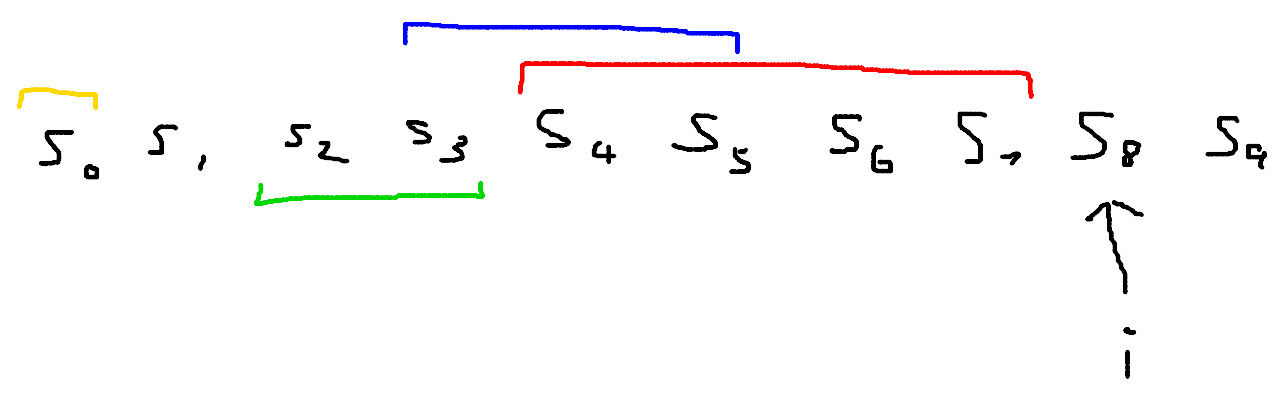
We are currently processing $i = 8$. The current linear recurrence sequence is the red one, is of length 4, and has just failed at index 8. We have three previous versions of $c$: a yellow sequence of length 1 that failed at index 1, a green sequence of length 2 that failed at index 4, and a blue sequence of length 3 that failed at index 6. You can also imagine there’s one more sequence: an empty sequence that failed at index 0. I didn’t draw it since it’s of length 0.
Let’s say we pick the blue sequence as our $b$. I have now drawn a purple segment on our diagram:
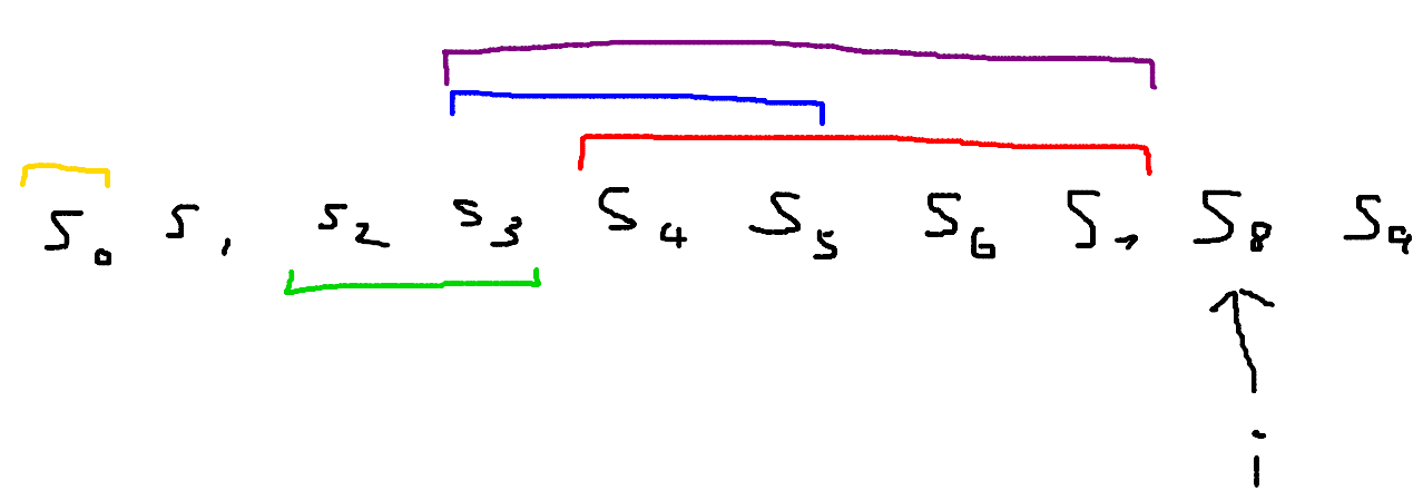
This purple segment represents the length of $d$. You can verify that one unit of increased length comes from the inserted 1, and one unit of increased length comes from the $i - f - 1 = 8 - 6 - 1 = 1$ zeros inserted. And the final updated $c’$ comes from overlaying the red and purple segments, representing us adding $c$ and $d$.
This tells us what the optimal $b$ is: the one whose segment has the rightmost left endpoint! So we only need to keep track of that best $c$ throughout the algorithm, not every previous version.
The First Step
Selecting a previous version of $c$ to use only works if you’re not updating $c$ for the first time. So what do you do if you do update $c$ for the first time? Let’s find out with the following example: $s = \{0, 0, 0, 0, 1, 0, 0, 2\}$. Once again, $c = \{\}$ initially.
Process $i = 0$. $c(0) = 0 = s_0$. So we keep going.
Process $i = 1$. $c(0) = 0 = s_1$. So we keep going.
This repeats until we reach $i = 4$. $c(0) = 0 \neq 1 = s_4$. Since we are updating $c$ for the first time, there are no previous versions of $c$ to rely on. So we will initialize $c$ to an arbitrary length 5 sequence. The reason why it must be at least length 5 is because that is the minimal length required to include $s_4$ in the base case. If $s_4$ was not part of the base case, then it must satisfy some recurrence $s_4 = \sum_{j=1}^n c_j s_{4-j}$. But since $s_0, s_1, s_2, s_3$ are all zero, such a recurrence would always evaluate to 0. So $s_4$ must be part of the base case. For simplicity, we will assign $c = \{0, 0, 0, 0, 0\}$, although like I stated in the previous example, the values could be arbitrary.
Now, when you update $c$ a second time when failing at index 7, you can rely on $b = \{\}$ with failure index 4. You can try by hand to confirm that this works.
What $c$ becomes at index 7
\[\{0, 0, 2, 0, 0\}\]Yes, the extra trailing 0s matter! Without them, $s_4$ would not be part of the base case!
Notice that if the sequence is all 0s, this algorithm will simply return $c = \{\}$, which is fine since we defined $c(i) = 0$ for an empty sequence.
Putting it all together in code…
1
2
3
4
5
6
7
8
9
10
11
12
13
14
15
16
17
18
19
20
21
22
23
24
25
26
27
28
29
30
31
32
33
34
35
36
37
38
39
40
41
42
43
44
45
46
47
48
49
50
51
52
53
54
55
56
57
58
59
60
61
template<typename T>
vector<T> berlekampMassey(const vector<T> &s) {
    vector<T> c;    // the linear recurrence sequence we are building
    vector<T> oldC; // the best previous version of c to use (the one with the rightmost left endpoint)
    int f = -1;     // the index at which the best previous version of c failed on
    for (int i=0; i<(int)s.size(); i++) {
        // evaluate c(i)
        // delta = s_i - \sum_{j=1}^n c_j s_{i-j}
        // if delta == 0, c(i) is correct
        T delta = s[i];
        for (int j=1; j<=(int)c.size(); j++)
            delta -= c[j-1] * s[i-j];   // c_j is one-indexed, so we actually need index j - 1 in the code
        if (delta == 0)
            continue;   // c(i) is correct, keep going
        // now at this point, delta != 0, so we need to adjust it
        if (f == -1) {
            // this is the first time we're updating c
            // s_i was the first non-zero element we encountered
            // we make c of length i + 1 so that s_i is part of the base case
            c.resize(i + 1);
            mt19937 rng(chrono::steady_clock::now().time_since_epoch().count());
            for (T &x : c)
                x = rng();  // just to prove that the initial values don't matter in the first step, I will set to random values
            f = i;
        } else {
            // we need to use a previous version of c to improve on this one
            // apply the 5 steps to build d
            // 1. set d equal to our chosen sequence
            vector<T> d = oldC;
            // 2. multiply the sequence by -1
            for (T &x : d)
                x = -x;
            // 3. insert a 1 on the left
            d.insert(d.begin(), 1);
            // 4. multiply the sequence by delta / d(f + 1)
            T df1 = 0;  // d(f + 1)
            for (int j=1; j<=(int)d.size(); j++)
                df1 += d[j-1] * s[f+1-j];
            assert(df1 != 0);
            T coef = delta / df1;   // storing this in outer variable so it's O(n^2) instead of O(n^2 log MOD)
            for (T &x : d)
                x *= coef;
            // 5. insert i - f - 1 zeros on the left
            vector<T> zeros(i - f - 1);
            zeros.insert(zeros.end(), d.begin(), d.end());
            d = zeros;
            // now we have our new recurrence: c + d
            vector<T> temp = c; // save the last version of c because it might have a better left endpoint
            c.resize(max(c.size(), d.size()));
            for (int j=0; j<(int)d.size(); j++)
                c[j] += d[j];
            // finally, let's consider updating oldC
            if (i - (int) temp.size() > f - (int) oldC.size()) {
                // better left endpoint, let's update!
                oldC = temp;
                f = i;
            }
        }
    }
    return c;
}
I tried to annotate the code as best as I can, using the same terminology as in the article. The method uses generic types, so you can plug in modint if you’re computing something under mod, or double, if you’re working with real numbers (warning that numerical stability is not guaranteed). If you need a working modint template, you can find mine here. The complexity of this algorithm is clearly $\mathcal O(n^2)$.
Test for Understanding
Do you really understand everything I just explained? If so, try your hand at some of these exercises! For the purpose of this exercise, assume the first step fills with $i + 1$ zeros instead of random values.
-
Find the intermediate sequences of $c$ after each step of the algorithm on $s = \{0, 2, 3, 4, 5, 6, 7, 8\}$.
Answer
$c$ after each $i$ is processed:
\[\begin{align*} i = 0&: c = \{\} \\ i = 1&: c = \{0, 0\} \\ i = 2&: c = \{3/2, 0\} \\ i = 3&: c = \{3/2, -1/4\} \\ i = 4&: c = \{3/2, -1/4, -1/8\} \\ i = 5&: c = \{2, -1, 0\} \\ i = 6&: c = \{2, -1, 0\} \\ i = 7&: c = \{2, -1, 0\} \end{align*}\]
-
Find the intermediate sequences of $c$ after each step of the algorithm on $s = \{1, 8, 10, 26, 46\}$.
Answer
$c$ after each $i$ is processed:
\[\begin{align*} i = 0&: c = \{0\} \\ i = 1&: c = \{8\} \\ i = 2&: c = \{8, -54\} \\ i = 3&: c = \{1, 2\} \\ i = 4&: c = \{1, 2\} \end{align*}\]
-
Find the intermediate sequences of $c$ after each step of the algorithm on $s = \{1, 3, 5, 11, 25, 59, 141, 339\}$.
Answer
$c$ after each $i$ is processed:
\[\begin{align*} i = 0&: c = \{0\} \\ i = 1&: c = \{3\} \\ i = 2&: c = \{3, -4\} \\ i = 3&: c = \{1, 2\} \\ i = 4&: c = \{1, 1, 3\} \\ i = 5&: c = \{3, -1, -1\} \\ i = 6&: c = \{3, -1, -1\} \\ i = 7&: c = \{3, -1, -1\} \end{align*}\]
Proofs
I know not everyone will be interested in this section, so I’ll put them under a spoiler.
Click Me!
The proofs come from Massey’s paper and will actually allow us to prove an even stronger condition on the minimum length recurrence relation, which will let us implement a conciser solution.
Definition: Let $L_i$ denote the minimum length recurrence relation for the prefix of the first $i$ elements of $s$. Let $r_i$ denote that recurrence relation of length $L_i$.
Theorem: If $r_{i-1}$ works for all positions up to $i - 1$ but not for position $i$ (i.e. $r_{i-1} \neq r_i$), then $L_i \geq \max(L_{i-1}, i + 1 - L_{i-1})$.
To prove this, we will prove the two arguments inside the $\max$ function separately.
Lemma 1: $L_i \geq L_{i-1}$
This lemma is kind of self-evident. By definition, $r_{i-1}$ must work for all positions up to $i - 1$ and is of minimal length for position $i - 1$. And $r_i$ must work for all positions up to $i$ and is of minimal length for position $i$. Say $L_i < L_{i-1}$. Then that contradicts the definition of $r_{i-1}$, because there exists a recurrence of shorter length that works for all positions up to $i - 1$: $r_i$. Notice that this lemma is true for all $i$, not just when $r_{i-1} \neq r_i$.
Lemma 2: $L_i \geq i + 1 - L_{i-1}$
Case 1: $L_{i-1} \geq i$
This case is self-evident, because then we get $L_i \geq 1$. There’s no way $L_i = 0$ because that would imply $r_i$ is the empty sequence. $L_{i-1}$ would also have to be 0 because $L_{i-1} \leq L_i$ and $L_{i-1}$ can’t be negative since you can’t have negative length. So $L_{i-1}$ would also have to be the empty sequence, and $r_{i-1} = r_i$, meaning the theorem no longer applies since the theorem assumes $r_{i-1}$ fails for position $i$.
Case 2: $L_{i-1} < i$
Let the coefficients of $r_{i-1}$ be $c_j$ and the coefficients of $r_i$ be $d_j$. By definition:
\[\sum_{j=1}^{L_{i-1}} c_j s_{k-j} \begin{cases} = s_k & L_{i-1} \leq k < i \\ \neq s_k & k = i \end{cases}\]and
\[\sum_{j=1}^{L_i} d_j s_{k-j} \begin{array}{cc} = s_k & L_i \leq k \leq i \end{array}\]We will do a proof by contradiction. Assume $L_i < i + 1 - L_{i-1}$. Thus,
\[\begin{align*} \sum_{j=1}^{L_{i-1}} c_j s_{i-j} &= \sum_{j=1}^{L_{i-1}} c_j \left( \sum_{k=1}^{L_i} d_k s_{i-j-k} \right) \\ &= \sum_{j=1}^{L_{i-1}} \sum_{k=1}^{L_i} c_j d_k s_{i-j-k} \\ &= \sum_{k=1}^{L_i} \sum_{j=1}^{L_{i-1}} d_k c_j s_{i-k-j} \\ &= \sum_{k=1}^{L_i} d_k \left( \sum_{j=1}^{L_{i-1}} c_j s_{i-k-j} \right) \\ &= \sum_{k=1}^{L_i} d_k s_{i-k} \\ &= s_i \end{align*}\]But this is a contradiction, since we forced by definition that $\sum_{j=1}^{L_{i-1}} c_j s_{i-j} \neq s_i$. Thus, $L_i \geq i + 1 - L_{i-1}$. Notice that the index $i - j - k$ never dips negative thanks to us assuming $L_i < i + 1 - L_{i-1}$.
Combining the above two lemmas provides us with our theorem.
Proving the Algorithm
We will initiate a proof by induction. Let the base case be the first position of a non-zero element in $s$ (if all the elements in $s$ are 0, the recurrence is just the empty sequence and we are done). As proven under “The First Step” section of this article, the optimal length of a first non-zero element at index $i$ is $i + 1$.
Now for the induction step: assume for all $j < i$, if $r_{j-1} \neq r_j$, then $L_j = \max(L_{j-1}, j + 1 - L_{j-1})$, and otherwise when $r_{j-1} = r_j$, then $L_j = L_{j-1}$. Then that same condition holds true for $j = i$. There are two cases.
Case 1: $r_{i-1}$ works for index $i$. In this case, we keep the same recurrence for the next index, and this is optimal per lemma 1.
Case 2: $r_{i-1}$ does not work for index $i$. Since this is not the first step, our algorithm chooses a previous version and use it to construct $d$. Recall from the section “Which $b$ do we choose?” that it is optimal to pick the version with the rightmost left endpoint. From here, we spawn two more cases:
Case 2a: The left endpoint of the old version is greater than or equal to the left endpoint of our current recurrence. In this case, the length of our new recurrence sequence does not change, which is optimal.
Case 2b: The left endpoint of the old version is less than the left endpoint of our current recurrence. In this case, the length of our new recurrence does change! Recall our theorem, which states that $L_i \geq \max(L_{i-1}, i + 1 - L_{i-1})$ when our recurrence changes. Since the length is getting longer, it must be that $L_i \geq i + 1 - L_{i-1}$. Let’s prove that our algorithm always yields $L_i = i + 1 - L_{i-1}$.
Let the index where our previous version failed be $m$. Notice that every time we update the previous version, it’s when the recurrence got longer. So $L_{m-1} < L_m = L_{m+1} = \dots = L_{i-1}$. By induction, $L_m = \max(L_{m-1}, m + 1 - L_{m-1})$. Since $L_m > L_{m-1}$, $L_m = m + 1 - L_{m-1}$, or $L_{m-1} = m + 1 - L_m = m + 1 - L_{i-1}$. Now, note that if the previous version failed at index $m$ and we are currently at index $i$, the length of the new recurrence will be $i - m + L_{m-1}$ (look at the diagram of segments above if you’re unsure). Finally,
\[\begin{align*} L_i &= i - m + L_{m-1} \\ &= i - m + (m + 1 - L_{i-1}) \\ &= i + 1 - L_{i-1} \end{align*}\]A More Concise Implementation
Our theorem above provided a stronger condition on $L_i$, which lets us greatly shorten our implementation. Take a look at the code below (courtesy of KACTL):
1
2
3
4
5
6
7
8
9
10
11
12
13
14
15
16
17
18
19
20
21
22
23
24
25
26
27
28
template<typename T>
vector<T> berlekampMassey(const vector<T> &s) {
    int n = (int) s.size(), l = 0, m = 1;
    vector<T> b(n), c(n);
    T ld = b[0] = c[0] = 1;
    for (int i=0; i<n; i++, m++) {
        T d = s[i];
        for (int j=1; j<=l; j++)
            d += c[j] * s[i-j];
        if (d == 0)
            continue;
        vector<T> temp = c;
        T coef = d / ld;
        for (int j=m; j<n; j++)
            c[j] -= coef * b[j-m];
        if (2 * l <= i) {
            l = i + 1 - l;
            b = temp;
            ld = d;
            m = 0;
        }
    }
    c.resize(l + 1);
    c.erase(c.begin());
    for (T &x : c)
        x = -x;
    return c;
}
Some notes about this implementation:
nis the length of the $s$ sequence, not the $c$ sequencecis our current recurrence relationbis our best previous versionlis the length of our current recurrence relationmis the number of steps since the last time we increased the length of our recurrence relationldis the last $\Delta$ computed with our previous version- In this implementation, we instead define the recurrence as $s_i + \sum_{j=1}^n c_j s_{i-j} = 0$, so we negate all the coefficients at the end.
- We also append a 1 at the beginning of
candb. You can figure out why this works by tracing the code. - This implementation also takes care of the first step, all with the same logic!
Applications in Problems
Ok, this is what you probably came for. Aside from contrived problems asking us to explicitly find the minimum length linear recurrence satisfying a sequence, what can we do with Berlekamp-Massey? The answer is that we pretty much never have to figure out an explicit recurrence ever again!
Take this Codeforces problem for example. First, let’s come up with a naive DP solution. Feel free to think for a while, then click the spoiler.
Naive DP Solution
Let $dp[i][a][b][c][d]$ be the number of chainwords of length $i$, where the final character in the chainword is the $b$th character of the $a$th word and the $d$th character of the $c$th word. Essentially, we maintain what segment we are on for the top and bottom hints. Let $L \leq 5$ be the maximum length of a dictionary word. The complexity of this algorithm is something like $\mathcal O(n^4 L^2 m)$, depending on how you implement your transitions.
This is obviously way too slow. But we can make the following observation: the transitions are the same for all $i$. When this is the case, we can turn the $m$ into a $\log m$ factor with matrix exponentation or the polynomial method. The number of states we have per $i$ is $\mathcal O(n^2 L^2) \leq 1600$. Matrix exponentiation will be too slow, but our new method using polynomials can handle this just fine!
Wait, this isn't a linear recurrence...
You’re right, when we look at the transition $dp[i][a][b][c][d] \to dp[i+1][e][f][g][h]$, this doesn’t look like a linear recurrence because the states have 5 dimensions instead of 1. I claim $\{dp[0][a][b][c][d], dp[1][a][b][c][d], \dots, dp[m][a][b][c][d]\}$ for any $a, b, c, d$ satisfies a linear recurrence of length $\mathcal O(n^2 L^2)$. I actually don’t know how to prove this claim, but I’ll include a train of thought I had below and maybe someone can let me know if that train leads anywhere. Who knows, maybe it’s not even true, although it seems to be true from past experience and self-generated examples.
First, we will convert our recurrence down to a 2D recurrence by compressing the indices. The technique for reducing a dimension is as follows. Say you have some 2D table $dp[i][j]$ with dimensions $n \times m$. You can instead express this as a 1D table $dp[i \cdot m + j]$ with dimension $n \cdot m$. Essentially, we express our 2D pair as a base $m$ number. Refer to the diagram below to see how the conversion from 2D to 1D coordinates works.
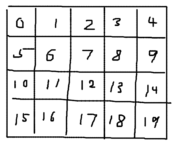
This same idea generalizes to multiple dimensions. For our example, $dp[a][b][c][d] \to dp[a \cdot L \cdot n \cdot L + b \cdot n \cdot L + c \cdot L + d]$.
So using this idea, we can compress $dp[i][a][b][c][d]$ down to 2 dimensions, $dp[i][\dots]$. We can express $dp[0], dp[1], \dots, dp[m]$ each as vectors of length $n^2 L^2$. For transitions, we can treat it as multiplying $dp[i]$ by some transition matrix $A$ of size $n^2 L^2 \times n^2 L^2$ to get $dp[i+1]$. And our desired result is $dp[m] = A^m dp[0]$.
The Cayley-Hamilton theorem states that if $A$ is of dimension $n \times n$, then $A^i$ satisfies a linear recurrence of length $n$ with coefficients of the characteristic polynomial. Specifically, it states $A^n = \sum_{j=1}^n c_j A^{n-j}$, and then we can generalize that to a linear recurrence for $A^i$ by multiplying both sides by $A^{i-n}$.
Now, I’m stuck, because I don’t think a linear recurrence for $A^m$ necessarily signifies a linear recurrence for a specific entry of $dp[m]$. If anyone knows something about this, I’d be dying to hear about it. As a bonus, it’s worth noting that you don’t have to rely on faith that a linear recurrence exists for a specific entry of $dp[m]$, and instead just compute $A^m dp[0]$ directly as explained in this blog. The idea is to generate some $1 \times n$ vector $\vec w$ to left multiply with $A^m dp[0]$ to convert from vector to scalar. Then, we can plug these scalar values into Berlekamp-Massey.
From here, showing a linear recurrence exists for $dp[m]$ can be done with some algebra. User shioko on Codeforces has worked out the details here.
Ok, so we know a linear recurrence of size $\mathcal O(n^2 L^2)$ exists, but what exactly is it? Let’s ask Berlekamp-Massey! Essentially, we will run the naive DP to generate the first few terms, then plug them into Berlekamp-Massey to get the full linear recurrence. It’s magic! Here’s a submission.
By the way, how many terms do we need to plug into Berlekamp-Massey before we can be sure we got the right recurrence? For example, say we’re working with the Fibonacci sequence $\{1, 1, 2, 3, 5, \dots\}$. If we just feed $\{1, 1, 2\}$ into Berlekamp-Massey, the algorithm could return $s_i = s_{i-1} + s_{i-2}$. But it could also return $s_i = 3s_{i-1} - s_{i-2}$. Or $s_i = 4s_{i-1} - 2s_{i-2}$. How do we ensure Berlekamp-Massey gives us the right recurrence?
It turns out, for a linear recurrence of length $n$, you need to feed at least $2n$ terms into Berlekamp-Massey to guarantee getting the same or equivalent recurrence.
Proof
Let’s say you only provide $2n - 1$ terms of the sequence. Say $n = 5$, the sequence is $\{0, 0, 0, 0, 1, 0, 0, 0, 0, 1, 0, 0, 0, 0, 1, \dots \}$, and the recurrence is $s_i = s_{i-5}$ for $i \geq 5$ (this counterexample is generalizable for any $n$). Another possible recurrence of length $n$ is $s_i = 0$ for $i \geq 5$ and base case $s_0 = s_1 = s_2 = s_3 = 0, s_4 = 1$. And we wouldn’t notice that this recurrence is wrong until we process $a_9$, or the $2n$th element.
On the other hand, if we have at least $2n$ elements, all $n$ length linear recurrences we could generate are equivalent. Say we have two recurrence sequences $c$ and $d$. We want to show if $s_i = \sum_{j=1}^n c_j s_{i-j} = \sum_{j=1}^n d_j s_{i-j}$ for $n \leq i < 2n$, then $s_i = \sum_{j=1}^n c_j s_{i-j} = \sum_{j=1}^n d_j s_{i-j}$ for all $i \geq 2n$ as well.
We initiate a proof by induction. The base case is $s_i = \sum_{j=1}^n c_j s_{i-j} = \sum_{j=1}^n d_j s_{i-j}$ for all $i < 2n$. Now for the induction step: if the condition is true for $i < k$, then the condition is true for $i = k$. Now we just crank out the math:
\[\begin{align*} s_k &= \sum_{j=1}^n c_j s_{k-j} \\ &= \sum_{j=1}^n c_j \left(\sum_{l=1}^n d_l s_{k-j-l} \right) \\ &= \sum_{j=1}^n \sum_{l=1}^n c_j d_l s_{k-j-l} \\ &= \sum_{l=1}^n \sum_{j=1}^n d_l c_j s_{k-l-j} \\ &= \sum_{l=1}^n d_l \left(\sum_{j=1}^n c_j s_{k-l-j} \right) \\ &= \sum_{l=1}^n d_l s_{k-l} \\ &= \sum_{j=1}^n d_j s_{k-j} \end{align*}\]Notice that $k - j - l$ never becomes negative since $k \geq 2n$, which is why this proof doesn’t work when we only provide $2n - 1$ or less elements for Berlekamp-Massey.
Now as an aside, it’s worth noting that in this problem, you need way less than $\mathcal O(n^2 L^2)$ terms. According to the editorial, there are only at most 241 states that matter, because we never reach certain combinations of states. Furthermore, in practice we don’t even need to calculate an exact bound. Since extra terms can’t hurt, it’s much easier to just generate as many terms as the problem’s time limit will allow, then plug all of them into Berlekamp-Massey and hope it gets AC. How easy is that?
Problems
While none of these problems require Berlekamp-Massey to solve, Berlekamp-Massey trivializes them significantly in my opinion.
Codeforces Round 286, Div 1 E: Mr. Kitayuta’s Gift
Atcoder Beginner Contest 198F: Cube
Codechef July Challenge 2021, PARTN01: Even Odd Partition
References
https://codeforces.com/blog/entry/61306
https://ieeexplore.ieee.org/stamp/stamp.jsp?arnumber=1054260